Download
1 / 43
430 likes | 542 Vues
Classical (frequentist) inference. Klaas Enno Stephan Laboratory for Social and Neural System Research Institute for Empirical Research in Economics University of Zurich Functional Imaging Laboratory (FIL) Wellcome Trust Centre for Neuroimaging University College London.

E N D
Classical (frequentist) inference Klaas Enno Stephan Laboratory for Social and Neural System Research Institute for Empirical Research in Economics University of Zurich Functional Imaging Laboratory (FIL) Wellcome Trust Centre for Neuroimaging University College London With many thanks for slides & images to: FIL Methods group Methods & models for fMRI data analysis in neuroeconomicsNovember 2010
Overview of SPM Statistical parametric map (SPM) Design matrix Image time-series Kernel Realignment Smoothing General linear model Gaussian field theory Statistical inference Normalisation p <0.05 Template Parameter estimates
model specification parameter estimation hypothesis statistic Voxel-wise time series analysis Time Time BOLD signal single voxel time series SPM
Overview • A recap of model specification and parameter estimation • Hypothesis testing • Contrasts and estimability • T-tests • F-tests • Design orthogonality • Design efficiency
Mass-univariate analysis: voxel-wise GLM X + y = • Model is specified by • Design matrix X • Assumptions about e N: number of scans p: number of regressors The design matrix embodies all available knowledge about experimentally controlled factors and potential confounds.
Parameter estimation Objective: estimate parameters to minimize = + X y Ordinary least squares estimation (OLS) (assuming i.i.d. error):
OLS parameter estimation The Ordinary Least Squares (OLS) estimators are: These estimators minimise . They are found solving either or Under i.i.d. assumptions, the OLS estimates correspond to ML estimates: NB: precision of our estimates depends on design matrix!
Maximum likelihood (ML) estimation probability density function ( fixed!) likelihood function (y fixed!) ML estimator For cov(e)=s2I, the ML estimator is equivalent to the OLS estimator: OLS For cov(e)=s2V, the ML estimator is equivalent to a weighted least sqaures (WLS) estimate (with W=V-1/2): WLS
SPM: t-statistic based on ML estimates c = 1 0 0 0 0 0 0 0 0 0 0 For brevity: ReML-estimates
Statistic • A statistic is the result of applying a mathematical function to a sample (set of data). • More formally, statistical theory defines a statistic as a function of a sample where the function itself is independent of the sample's distribution. The term is used both for the function and for the value of the function on a given sample. • A statistic is distinct from an unknown statistical parameter, which is a population property and can only be estimated approximately from a sample. • A statistic used to estimate a parameter is called an estimator. For example, the sample mean is a statistic and an estimator for the population mean, which is a parameter.
Null Distribution of T Hypothesis testing To test an hypothesis, we construct a “test statistic”. • “Null hypothesis” H0 = “there is no effect” cT = 0 This is what we want to disprove. The “alternative hypothesis” H1 represents the outcome of interest. • The test statistic T • The test statistic summarises the evidence for H0. • Typically, the test statistic is small in magnitude when H0 is true and large when H0 is false. • We need to know the distribution of T under the null hypothesis.
Hypothesis testing • Type I Error α: • Acceptable false positive rate α. • Threshold uα controls the false positive rate u • Observation of test statistic t, a realisation of T: • A p-value summarises evidence against H0. • This is the probability of observing t, or a more extreme value, under the null hypothesis: Null Distribution of T t • The conclusion about the hypothesis: • We reject H0 in favour of H1 if t > uα p Null Distribution of T
False positive (FP) Type I error False negative (FN) Type II error β Types of error Actual condition H0 true H0 false True positive (TP) Reject H0 Test result Failure to reject H0 True negative (TN) specificity: 1- = TN / (TN + FP) = proportion of actual negatives which are correctly identified sensitivity (power): 1- = TP / (TP + FN) = proportion of actual positives which are correctly identified
One cannot accept the null hypothesis(one can just fail to reject it) Absence of evidence is not evidence of absence! If we do not reject H0, then all can we say is that there is not enough evidence in the data to reject H0. This does not mean that we can accept H0. What does this mean for neuroimaging results based on classical statistics? A failure to find an “activation” in a particular area does not mean we can conclude that this area is not involved in the process of interest.
Contrasts • We are usually not interested in the whole vector. • A contrast cT selects a specific effect of interest: a contrast vector c is a vector of length p cTis a linear combination of regression coefficients cT = [1 0 0 0 0 …] cTβ = 1b1 + 0b2 + 0b3 + 0b4 + 0b5 + . . . cT = [0 -1 1 0 0 …] cTβ = 0b1+-1b2 + 1b3 + 0b4 + 0b5 + . . . • Under i.i.d assumptions: NB: the precision of our estimates depends on design matrix and the chosen contrast !
1 2 Factor Factor Mean images parameters parameter estimability ® not uniquely specified) (gray b Estimability of parameters • If X is not of full rank then different parameters can give identical predictions, i.e. Xb1 = Xb2 with b1≠b2. • The parameters are therefore ‘non-unique’, ‘non-identifiable’ or ‘non-estimable’. • For such models, XTX is not invertible so we must resort to generalised inverses (SPM uses the Moore-Penrose pseudo-inverse). • This gives a parameter vector that has the smallest norm of all possible solutions. One-way ANOVA(unpaired two-sample t-test) 1 0 1 1 0 1 1 0 1 1 0 1 0 1 1 0 1 1 0 1 1 0 1 1 Rank(X)=2 • However, even when parameters are non-estimable, certain contrasts may well be!
Estimability of contrasts • Linear dependency: there is one contrast vector q for which Xq= 0. • Thus: y = Xb+Xq+e = X(b+q)+e • So if we test cTb we also test cT(b+q), thus an estimable contrast has to satisfy cTq = 0. • In the above example, any contrast that is orthogonal to [1 1 -1] is estimable: [1 0 0], [0 1 0], [0 0 1] are not estimable. [1 0 1], [0 1 1], [1 -1 0], [0.5 0.5 1] are estimable.
0.4 n =1 0.35 n =2 n =5 0.3 n =10 n ¥ = 0.25 0.2 0.15 0.1 0.05 0 -5 -4 -3 -2 -1 0 1 2 3 4 5 Probability density function of Student’s t distribution Student's t-distribution • first described by William Sealy Gosset, a statistician at the Guinness brewery at Dublin • t-statistic is a signal-to-noise measure: t = effect / standard deviation • t-distribution is an approximation to the normal distribution for small samples • t-contrasts are simply combinations of the betas the t-statistic does not depend on the scaling of the regressors or on the scaling of the contrast • Unilateral test: vs.
contrast ofestimatedparameters t = varianceestimate t-contrasts – SPM{t} box-car amplitude > 0 ? = H1 = cTb > 0 ? Question: cT = 1 0 0 0 0 0 0 0 b1b2b3b4b5 ... H0: cTb=0 Null hypothesis: Test statistic:
t-contrasts in SPM For a given contrast c: ResMS image beta_???? images spmT_???? image con_???? image SPM{t}
Statistics: 1 p-values adjusted for search volume set-level cluster-level voxel-level mm mm mm p c p k p p p T Z p ( ) corrected E uncorrected FWE-corr FDR-corr uncorrected º 0.000 10 0.000 520 0.000 0.000 0.000 13.94 Inf 0.000 -63 -27 15 SPMresults: 0.000 0.000 12.04 Inf 0.000 -48 -33 12 0.000 0.000 11.82 Inf 0.000 -66 -21 6 10 Height threshold T = 3.2057 {p<0.001} 0.000 426 0.000 0.000 0.000 13.72 Inf 0.000 57 -21 12 0.000 0.000 12.29 Inf 0.000 63 -12 -3 0.000 0.000 9.89 7.83 0.000 57 -39 6 20 0.000 35 0.000 0.000 0.000 7.39 6.36 0.000 36 -30 -15 0.000 9 0.000 0.000 0.000 6.84 5.99 0.000 51 0 48 0.002 3 0.024 0.001 0.000 6.36 5.65 0.000 -63 -54 -3 0.000 8 0.001 0.001 0.000 6.19 5.53 0.000 -30 -33 -18 30 0.000 9 0.000 0.003 0.000 5.96 5.36 0.000 36 -27 9 0.005 2 0.058 0.004 0.000 5.84 5.27 0.000 -45 42 9 0.015 1 0.166 0.022 0.000 5.44 4.97 0.000 48 27 24 40 0.015 1 0.166 0.036 0.000 5.32 4.87 0.000 36 -27 42 50 60 70 80 0.5 1 1.5 2 2.5 Design matrix t-contrast: a simple example Passive word listening versus rest cT = [ 1 0 ] Q: activation during listening ? Null hypothesis:
X0 X0 X1 RSS RSS0 Or reduced model? F-test: the extra-sum-of-squares principle Model comparison: Full vs. reduced model Null Hypothesis H0: True model is X0(reduced model) F-statistic: ratio of unexplained variance under X0 and total unexplained variance under the full model 1 = rank(X) – rank(X0) 2 = N – rank(X) Full model (X0 + X1)?
0 0 1 0 0 0 0 0 0 0 0 1 0 0 0 0 0 0 0 0 1 0 0 0 0 0 0 0 0 1 0 0 0 0 0 0 0 0 1 0 0 0 0 0 0 0 0 1 cT = F-test: multidimensional contrasts – SPM{F} Tests multiple linear hypotheses: H0: True model is X0 H0: b3 = b4 = ... = b9 = 0 test H0 : cTb = 0 ? X0 X0 X1 (b3-9) SPM{F6,322} Full model? Reduced model?
F-test: a few remarks • F-tests can be viewed as testing for the additional variance explained by a larger model wrt. a simpler (nested) model model comparison • Hypotheses: Null hypothesis H0:β1 = β2 = ... = βp = 0 Alternative hypothesis H1: At least one βk ≠ 0 • F-tests are not directional:When testing a uni-dimensional contrast with an F-test, for example b1 – b2, the result will be the same as testing b2 – b1.
F-contrast in SPM ResMS image beta_???? images ess_???? images spmF_???? images ( RSS0 - RSS) SPM{F}
F-test example: movement related effects To assess movement-related activation: There is a lot of residual movement-related artifact in the data (despite spatial realignment), which tends to be concentrated near the boundaries of tissue types. By including the realignment parameters in our design matrix, we can “regress out” linear components of subject movement, reducing the residual error, and hence improve our statistics for the effects of interest.
True signal (--) and observed signal Model (green, peak at 6sec) TRUE signal (blue, peak at 3sec) Fitting (b1 = 0.2, mean = 0.11) Residuals(still contain some signal) Example: a suboptimal model Test for the green regressor not significant
Example: a suboptimal model b1= 0.22 b2= 0.11 Residual Var.= 0.3 p(Y|b1= 0) p-value = 0.1 (t-test) p(Y|b1= 0)p-value = 0.2 (F-test) = + Y X b e
True signal + observed signal Model (green and red) and true signal (blue ---) Redregressor: temporal derivative of the greenregressor Total fit (blue) and partial fit (green & red) Adjusted and fitted signal Residuals (less variance & structure) A better model t-test of the green regressor almost significant F-test very significant t-test of the red regressor very significant
A better model b1= 0.22 b2= 2.15 b3= 0.11 Residual Var. = 0.2 p(Y|b1= 0) p-value = 0.07 (t-test) p(Y|b1= 0, b2= 0) p-value = 0.000001 (F-test) = + Y X b e
Correlation among regressors y x2 x2* x1 Correlated regressors = explained variance is shared between regressors When x2 is orthogonalized with regard to x1, only the parameter estimate for x1 changes, not that for x2!
Design orthogonality • For each pair of columns of the design matrix, the orthogonality matrix depicts the magnitude of the cosine of the angle between them, with the range 0 to 1 mapped from white to black. • The cosine of the angle between two vectors a and b is obtained by: • If both vectors have zero mean then the cosine of the angle between the vectors is the same as the correlation between the two variates.
Correlated regressors True signal Model (green and red) Fit (blue : total fit) Residual
Correlated regressors b1 = 0.79 b2 = 0.85 b3 = 0.06 Residual var. = 0.3 p(Y|b1= 0) p-value = 0.08 (t-test) P(Y|b2= 0) p-value = 0.07 (t-test) p(Y|b1= 0, b2= 0) p-value = 0.002 (F-test) = + Y X b e 1 2 1 2
Model (green and red) red regressor has been orthogonalised with respect to the green one remove everything that correlates with the green regressor After orthogonalisation True signal Fit (does not change) Residuals (do not change)
1 2 After orthogonalisation b1 = 1.47 b2 = 0.85 b3 = 0.06 (0.79) (0.85) (0.06) Residual var. = 0.3 p(Y|b1= 0) p-value = 0.0003 (t-test) p(Y|b2= 0) p-value = 0.07 (t-test) p(Y|b1= 0, b2= 0) p-value = 0.002 (F-test) does change = + does not change does not change Y X b e 1 2
Design efficiency • The aim is to minimize the standard error of a t-contrast (i.e. the denominator of a t-statistic). • This is equivalent to maximizing the efficiency ε: Noise variance Design variance • If we assume that the noise variance is independent of the specific design: NB: efficiency depends on design matrix and the chosen contrast ! • This is a relative measure: all we can say is that one design is more efficient than another (for a given contrast).
Design efficiency • XTX is the covariance matrix of the regressors in the design matrix • efficiency decreases with increasing covariance • but note that efficiency differs across contrasts cT = [1 0] →ε = 0.19 cT = [1 1] →ε = 0.05 cT = [1 -1] →ε = 0.95 blue dots: noise with the covariance structure of XTX
Example: working memory A B C Stimulus Stimulus Stimulus Response Response Response • A: Response follows each stimulus with (short) fixed delay. • B: Jittering the delay between stimuli and responses. • C: Requiring a response only for half of all trials (randomly chosen). Time (s) Correlation = -.65Efficiency ([1 0]) = 29 Correlation = +.33Efficiency ([1 0]) = 40 Correlation = -.24Efficiency ([1 0]) = 47
Bibliography • Friston KJ et al. (2007) Statistical Parametric Mapping: The Analysis of Functional Brain Images. Elsevier. • Christensen R (1996) Plane Answers to Complex Questions: The Theory of Linear Models. Springer. • Friston KJ et al. (1995) Statistical parametric maps in functional imaging: a general linear approach. Human Brain Mapping 2: 189-210. • Mechelli A et al. (2003) Estimating efficiency a priori: a comparison of blocked and randomized designs. NeuroImage 18:798-805.
Differential F-contrasts • equivalent to testing for effects that can be explained as a linear combination of the 3 differences • useful when using informed basis functions and testing for overall shape differences in the HRF between two conditions