Download
1 / 112
1.13k likes | 1.3k Vues
Data Structures. CSC 336. Definition. Data structures are the physical implementations of data storage. Different structures are better for different types of problems.

E N D
Data Structures CSC 336
Definition • Data structures are the physical implementations of data storage. Different structures are better for different types of problems. • There are three fundamental abstract data types. Data structures implement these and there are lots more than three of those. Let’s take a look…
Elementary Data Structures “Mankind’s progress is measured by the number of things we can do without thinking.” Elementary data structures such as stacks, queues, lists, and heaps are the “off-the-shelf” components we build our algorithm from. There are two aspects to any data structure: • The abstract operations which it supports. • The implementation of these operations.
Data Abstraction • We can define our data structures in terms of abstract operations they can perform. • We optimize performance by a careful choice of which data structure works the best with our problem.
Contiguous vs. Linked Data Structures Data structures can be neatly classified as either contiguous or linked depending upon whether they are based on arrays or pointers: • Contiguously-allocated structures are composed of single slabs of memory, and include arrays, matrices, heaps, and hash tables. • Linked data structures are composed of multiple distinct chunks of memory bound together by pointers, and include lists, trees, and graph adjacency lists.
Arrays • Who’s heard of them? • Who’s used them? • Who can describe them? • What are their drawbacks?
Arrays An array is a structure of fixed-size data records such that each element can be efficiently located by its index or (equivalently) address. Advantages of contiguously-allocated arrays include: • Constant-time access given the index. • Arrays consist purely of data, so no space is wasted with links or other formatting information. • Physical continuity (memory locality) between successive data accesses helps exploit the high-speed cache memory on modern computer architectures.
Dynamic Arrays • Unfortunately we cannot adjust the size of simple arrays in the middle of a program’s execution. • Compensating by allocating extremely large arrays can waste a lot of space. • With dynamic arrays we start with an array of size 1, and double its size from m to 2m each time we run out of space. • How many times will we double for n elements? Only (ceiling of)(log2 n).
Pointers and Linked Structures • Pointers represent the address of a location in memory. • A cell-phone number can be thought of as a pointer to its owner as they move about the planet. • In C, *p denotes the item pointed to by p, and &x denotes the address (i.e. pointer) of a particular variable x. • A special NULL pointer value is used to denote structure-terminating or unassigned pointers.
Searching a List • Can be done iteratively or recursively
Insertion into a List • Since we have no need to maintain the list in any particular order, we might as well insert each new item at the head.
Advantages of Linked Lists The relative advantages of linked lists over static arrays include: 1. Overflow on linked structures can never occur unless the memory is actually full. 2. Insertions and deletions are simpler than for contiguous (array) lists. 3. With large records, moving pointers is easier and faster than moving the items themselves. Dynamic memory allocation provides us with flexibility on how and where we use our limited storage resources.
Stacks and Queues • Sometimes, the order in which we retrieve data is independent of its content, being only a function of when it arrived. • A stack supports last-in, first-out operations: push and pop. • A queue supports first-in, first-out operations: enqueueand dequeue. • Lines in banks are based on queues, while food in my refrigerator is treated as a stack.
Dictonary / Dynamic Set Operations Perhaps the most important class of data structures maintain a set of items, indexed by keys. • Search(S,k) – A query that, given a set S and a key value k, returns a pointer x to an element in S such that key[x] = k, or nil if no such element belongs to S. • Insert(S,x) – A modifying operation that augments the set S with the element x. • Delete(S,x) – Given a pointer x to an element in the set S, remove x from S. Observe we are given a pointer to an element x, not a key value. • Min(S), Max(S) – Returns the element of the totally ordered set S which has the smallest (largest) key. • Next(S,x), Previous(S,x) – Given an element x whose key is from a totally ordered set S, returns the next largest (smallest) element in S, or NIL if x is the maximum (minimum) element. There are a variety of implementations of these dictionary operations, each of which yield different time bounds for various operations.
Array Based Sets: Unsorted Arrays • Search(S,k) - sequential search, O(n) • Insert(S,x) - place in first empty spot, O(1) • Delete(S,x) - copy nth item to the xth spot, O(1) • Min(S,x), Max(S,x) - sequential search, O(n) • Successor(S,x), Predecessor(S,x) - sequential search, O(n)
Array Based Sets: Sorted Arrays • Search(S,k) - binary search, O(lg n) • Insert(S,x) - search, then move to make space, O(n) • Delete(S,x) - move to fill up the hole, O(n) • Min(S,x), Max(S,x) - first or last element, O(1) • Successor(S,x), Predecessor(S,x) - Add or subtract 1 from pointer, O(1)
Pointer Based Implementation • We can maintain a dictionary in either a singly or doubly linked list.
Doubly Linked Lists • We gain extra flexibility on predecessor queries at a cost of doubling the number of pointers by using doubly-linked lists. • Since the extra big-Oh costs of doubly-linkly lists is zero, we will usually assume they are, although it might not be necessary. • Singly linked to doubly-linked list is as a Conga line is to a Can-Can line.
Trees There are two general forms of trees: • Binary Trees • General How do we use trees?
Concepts What if we need to categorize our data into groups and subgroups, not in linear order? A queue or stack is not set up for this. This hierarchical classification appears often in problems and we should be able to represent it.
Other CS Uses for Trees • Folders/files on a computer • Each folder/file is a node, subfolders are children. • AI: decision trees / game trees • Compilers: parse tree a = (b + c) * d; • Expression Trees
Trees • So, what exactly is a tree?
Terminology Tree – set of nodes connected by edges that indicate the relationships among the nodes. Nodes are arranged in levels that indicate the node’s hierarchy. The top level is a single node called the root.
Terminology • Trees have a starting node called the root; all other nodes are reachable from the root by the edges between them. • GOAL: Use a tree to build a collection that has O(log n) time for many useful operations.
Terminology • Nodes at each successive level of a tree are the children of the nodes at the previous level. • A node that has children is the parent of those children • Nodes with the same parent are called siblings. • Nodes can also be ancestors and/or descendants.
Terminology • Nodes with no children are called leaf nodes. • Nodes with children are called interior nodes or non-leaf nodes. • Any node and its descendants form a subtree of the original tree.
r T2 T3 T1 Visualizing Trees • every node links to a set of subtrees • root of each subtree is a child of root r. • r is the parent of each subtree.
Terminology • The height of the tree is the number of levels of the tree. • The height of a node is the length of the path from the node to the deepest leaf. • We can reach any node in a tree by following a path that begins at the root and goes from node to node along the edges that join them. The path between the root and any other node is unique.
Terminology • The length of a path is the number of edges that compose it (which is one less than the number of nodes in the path). • The depth of a node is the length of the path from the root to the node. • The depth of any node is one more than the depth of its parent.
Paths • path: a sequence of nodes n1, n2, … , nk such that ni is the parent of ni+1 for 1 i < k • in other words, a sequence of hops to get from one node to another • the length of a path is the number of edges in the path, or 1 less than the number of nodes in it
Depth and Height • depth or level: length of the path from root to the current node (depth of root = 0) • height: length of the longest path from root to any leaf • empty (null) tree's height: -1 • single-element tree's height: 0 • tree with a root with children: 1
Trees • General Trees: Each node in the tree can have an arbitrary number of children • n-ary tree: Each node has no more than “n” children • Binary tree: Each node has no more than 2 children.
Binary Trees • Each node has at most two children. • Children are called the left child and the right child. • Root of a binary tree has two subtrees – the left subtree and the right subtree. • Every subtree in a binary tree is also a binary tree.
1 2 3 4 5 6 7 Binary Trees • When a binary tree of height h has all of its leaves at level h and every non-leaf has exactly two children, the tree is said to be full. • If all levels of the binary tree contain as many nodes as possible and the nodes on the last level are filled from left to right, the tree is complete.
Fact • The height of a binary tree with n nodes that is either complete or full is (floor of)(log2n).
Traversals • Aka “iteration” • We must “visit” or process each node exactly once. • Order in which we visit is not unique. We can choose an order suitable to our application. • “Visiting” a node means to “process the data within” that node.
Traversals of a Binary Tree • We know that each subtree of a binary tree is a binary tree. • We can use recursion to visit all the nodes. • To visit all, we must visit the root, visit all nodes in the left subtree (LST) and all nodes in the right subtree (RST)
Common Traversals • Preorder (Root,Left,Right) • Depth-first traversal • Inorder (Left, Root, Right) • Postorder (Left, Right, Root) • Level-order – visits nodes from left to right within each level of the tree, beginning with the root • Breadth-first traversal
Preorder Traversal (Root, Left, Right) • order: ??
Preorder Traversal (Root, Left, Right) • order: 1,2,4,8,9,5,10,11,3,6,12,13,7,14,15
Inorder Traversal (Left, Root, Right) • order: ??
Inorder Traversal (Left, Root, Right) • order: 8,4,9,2,10,5,11,1,12,6,13,3,14,7,15
Postorder Traversal (Left, Right, Root) • order: ??