Download
1 / 48
780 likes | 1.49k Vues
Summary. : GVD; :TOD. When fiber loss/gain and TOD are neglected and is a constant independent of z, the above equation is known as the nonlinear Schrodinger equation (NSE), which has soliton solutions when dispersion is anomalous (negative or positive D).

E N D
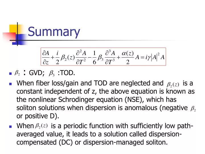
Summary • : GVD; :TOD. • When fiber loss/gain and TOD are neglected and is a constant independent of z, the above equation is known as the nonlinear Schrodinger equation (NSE), which has soliton solutions when dispersion is anomalous (negative or positive D). • When is a periodic function with sufficiently low path-averaged value, it leads to a solution called dispersion-compensated (DC) or dispersion-managed soliton.
Multiple Pulses Interaction • DWDM, interchannel four-wave mixing (FWM) and XPM; • High-speed TDM, intrachannel FWM and XPM.
Outline • Different Propagation Regimes • Dispersion-Induced Pulse Broadening • Fiber Transfer Function • Gaussian Pulses • Chirped Gaussian Pulses • Hyperbolic-Secant Pulses • Super Gaussian Pulses • Third-Order Dispersion • Broadening Factor • Dispersion Management • Dispersion Compensation
Different Propagation Regimes • For pulse width >5 ps (spectral width > 0.1 THz): • Normalized time scale t: • Normalized amplitude U: (1) (2)
Dispersion Length and Nonlinear Length • Dispersion Length LD: • Nonlinear Length LNL: • Fiber Length L<<LNL and L<<LD, neither dispersive nor nonlinear effects play a significant role. The pulse maintains its shape during propagation, i.e., • If L<<LNL but L~LD, the pulse evolution is governed by GVD. • If L<<LD but L~LNL, the pulse evolution is governed by SPM. • If L>LD and L>LNL, the pulse evolution is governed by GVD and SPM.
Wave Equation for the Envelope Function • The propagation constant: • The wave envelope function is a slowly varying function in z and t:
Generalized Schroedinger Equation • The correspondence: • Keep the terms up to the second order:
Generalized Schroedinger Equation • Retarded Frame (the frame of reference moving with the pulse at the group velocity vg: • Similar to the paraxial wave equation that governs diffraction of cw light (Space-Time Duality). • Similar to diffusion equation.
Fiber Transfer Function • Introduce a normalized amplitude U:
Gaussian Pulse T0: 1/e-intensity point. Full-Width-at-Half-Maximum:
Gaussian Pulses 1. Take the Fourier transform of U(0, T): 2. Find the output field U(z, w): 3. Take the inverse Fourier transform of U(z, w): Broadening factor: The fiber imposes linear frequency chirp on the pulse.
GVD-Induced Pulse Broadening • Fiber imposes linear frequency chirp on the pulse. • In the normal-dispersion regime (GVD>0), the chirp is negative at the leading edge (T<0) and increases linearly across the pulse. • In the anomalous-dispersion regime (GVD<0), the chirp is positive at the leading edge and decreases across the pulse. • Different frequency components of a pulse travel at slightly different speeds along the fiber because of GVD. • Red components travel faster than blue components in the normal-dispersion regime (GVD>0); • Blue components travel faster than red components in the anomalous-dispersion regime (GVD<0);
Pulse Broadening in 2.5-km-Long Fiber due to Dispersion L. Cohen W. Mammel, and H. Presby, “Correlation between numerical predictions and measurements of single-mode fiber dispersion characteristics,” Appl. Opt. 19, 2007 (1980).
Unchirped and Chirped Pulses • An unchirped input pulse with a Gaussian envelope. The spectral width is transform-limited and satisfies • The pulse after propagation in a dispersive fiber (b2<0) is chirped. The spectral width is enhanced by in the presence of linear chirp. • The pulse is broader and is chirped after propagation in a fiber.
Chirped Gaussian Pulses C is a chirp parameter. Broadening factor: 1. 2. 3. If b2C>0, the pulse broadens monotonically with z. If b2C<0, the pulse goes initially narrowing. When , the minimum pulse width: The pulse is Fourier-transform-limited
Impact of GVD on Pulse Broadening • When the pulse is initially chirped and the condition is satisfied, the dispersion-induced chirp is opposite direction to that of the initial chirp. • The net chirp is reduced, leading to pulse narrowing. The minimum pulse width occurs at a point at which the two chirps cancel each other. With further increase in the propagation distance, the dispersion-induced chirp starts to dominate over the initial chirp, and the pulse begins to broaden.
Hyperbolic-Secant Pulses 1. Take the Fourier transform of U(0, T): 2. Find the output field U(z, w): 3. Take the inverse Fourier transform of U(z, w):
Pulse Broadening at Different Chirp Coefficients • Broadening faster with the increase of C.
Super-Gaussian Pulses 1. Take the Fourier transform of U(0, T): 2. Find the output field U(z, w): 3. Take the inverse Fourier transform of U(z, w):
Broadening Factor • Pulse width: • For Super-Gaussian Pulses:
Super-Gaussian Pulse Shapes • Pulse distortion. • Broadening faster with increase of m.
Third-Order Dispersion • Zero-dispersion wavelength lD, b2~0; • Ultra-short Pulses: T0<1ps.
Changes in Pulse Shapes Gaussian Pulse Super-Gaussian Pulse • Asymmetry with an oscillatory structure near the edges; • b3>0, the oscillations appear near the trailing edge; • b3<0, the oscillations appear near the leading edge; • b2=0, the oscillations are deep.
General Case: Higher Order Dispersion • General case including higher order M Amemiya, “Pulse Broadening due to Higher Order Dispersion and its Transmission Limit”, Journal of Lightwave Technology, Vol 20, No 4, 591-597 (2002).
Arbitrary-Shape Pulses • Arbitrary shape and high order dispersion D Anderson and M Lisak, “Analytic study of pulse broadening in dispersive optical fibers”, Phys Rev A 35 (1), 184-187 (1987).
Dispersion Compensation • Spectral shaping at the transmitter; • Pre-chirping • Data Recovery at the receiver; • The Optical Regime: • Interferometers • Fiber Grating • Negative-Dispersion Fiber • Optical Phase Conjugation:OFC (Spectral Inversion)
Interferometer for Dispersion Compensation • 1-cm-long FP cavity, r=0.8,
Fiber Bragg Grating Af Ab
Chirped Fiber Grating • D=-8000ps/nm Ouellette F.(1987). Dispersion cancellation using linearly chirped Bragg grating filters in optical waveguides. Opt Lett. 12, 847.
Dispersion Compensated Fiber • Dispersion Compensation condition:
Dispersion Compensating Fiber (DCF) 1. 2. 3. If The output pulse is identical in form and width to that of the input.
Optical Phase Conjugation Optical phase conjugator Pump Input Output Four-wave mixing: The conjugator inverts all the optical frequencies about w0. Yariv, “Optical Electronics in Modern Communications”, (Oxford University Press, 1997), Chap. 3. Changxi Yang, “Dispersion compensation for a femtosecond self-pumped phase conjugator”, Opt. Lett., 24, 31(1999). Changxi Yang, J. Opt Soc Am B, 16, 871 (1999).
Dispersion Compensation by OFC: Principle • The pulse shape is completely recovered.
Dispersion Compensation by OPC: Principle 1. 2. 3. 4. If we choose the two fibers such that: The output envelope is identical to that of the input.
Compensation of Self-Phase Modulation • SPM-induced phase shift is power dependent. • When a=0, Midspan OPC can compensate for SPM and GVD simultaneously. • When , SPM cannot be compensated completely. Where Only if Perfect SPM compensation by OPC.