Download
1 / 87
870 likes | 898 Vues
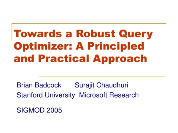
This paper presents a principled and practical approach to optimizing queries in database systems. It addresses the limitations of traditional query optimizers and proposes improvements using techniques like random sampling and confidence thresholds. By incorporating probability distributions of selectivity into the optimization process, it achieves more accurate cost estimates and better query performance. The use of sampling methods helps in estimating selectivity and query costs with greater accuracy, leading to improved database system performance and scalability.

E N D
Towards a Robust Query Optimizer: A Principled and Practical Approach Brian Badcock Surajit Chaudhuri Stanford University Microsoft Research SIGMOD 2005
目录 • 研究背景 • 传统查询优化器的问题 • 论文的解决方案 • 对查询优化器的改进 • 随机sampling • 置信度阈值 • 分析 • 总结
研究背景 • 传统查询优化器的问题 • 传统的查询计划的代价估算 • 属性值的独立性( Attribute value independence) • 在很多情况下表中列的取值是独立的 • 多维属性值分布的描述 • Multidimensional Histograms • Graphical models • 随着维度的增加,桶的数量呈指数级增长( curse of dimensionality) • 假设估计的结果是正确的,
本文的出发点 • Selectivity的估测是满足一个分布的 • 不同的访问计划在不同的Selectivity下是不同 • 嵌套循环join • Selectivity低的情况下代价较大 • 代价比较稳定 • Index join • Selectivity低的情况下代价较小 • 代价不稳定 • 采用Sample的方法
技术途径 • 需要解决的问题 • Selectivity的概率分布如何应用于查询优化 • 如何得到概率分布 • 论文的思路 • 评估方法对数据库系统的体系结构没有影响 • 使用SAMPLE的方法进行代价分析的好处 • 使用SAMPLE的方法描述查询的Selectiviy
基于概率分布的查询优化 • 假设:能够获得针对Selectivity的代价概率分布 • 两种方案的比较 • 平均代价 • 最坏代价 • Confidence threshold • 有T%的可能性最终的计算代价小于估计的结果 • 累计分布函数(cumulative distribution function) • CDF(Y)=
Dealing with Predictability • If we look at the distributions, we see that Plan 2 hits 80% of all plans (all execution patterns) with a cost of 31.9. Plan 1 only hits 80% of all plans at a cost of 33.5.
查询代价概率密度函数的计算方法 • 信息源 • Selectivity的概率密度函数:f(s) • 针对特定Selectivity的计算代价:c=g(s) • 计算公式
SAMPLE的方法 • 随机SAMPLE的优点 • 不受AVI的影响 • 不受“Curse of dimensionality”的影响 • 不受Equality和range谓词的限制 • 易于操作 • 两步工作 • 预计算 • 通过Update Statistics命令执行 • 估测 • 在查询优化的过程中执行
Joins SELECT * FROM INVENTORY inv, PRICE p WHERE inv.count >= 30 AND p.price < 1400 AND inv.model = p.model
Joins - Synopsis • Select a sample from INVENTORY: (hp,40), (asus,20). • Join sample with PRICES. We get results (HP,40,99), (ASUS, 20, 1500). This new sample captures the foreign key relationship between the two tables. We run out join on this sample.
代价评估阶段 • 通过对采样的结果进行直接计算获得Selectivity的结果 • 对A and B and C需要生成各种组合的Selectivity • 优点 • 避免了AVI假设 • 不存在高维的问题 • 对各种查询均有效 • 操作简单
生成概率分布函数 • 对N条元组的表T,取其一个采样S=s1,s2,…, sn (采用随机采样的方法)。对谓词P,X=(x1, x2,…,xn)是一个向量,xi代表si是否满足谓词P。求满足T中满足P的比例p。需要计算p的概率分布。等价于求条件密度函数f(z|X)。
生成概率分布函数 • f(z)的两种处理方法 • 通过背景知识(selecity在实际运行中的分布)进行推算 • 基于采样的结果进行推测,selectivity的分布符合beta分布参数是(1/2,1/2) • 公式其他的部分 • Pr[X|p=z]= zk(1-z)n-k
Results • Picking a low confidence threshold leads to large fluctuations in query execution time.
Conclusions • We want to be able to ask the optimizer to provide not just fast plans, but plans with predictable performance. • Having a large confidence threshold improves predictability, but can also help execution time! • Running queries on static samples is a nice compromise between keeping very detailed histograms and runtime sampling.
Discussion • Join synopsis seems to help estimates, but it is applied here in only a very restricted case (foreign key trees). • Not clear how well this approach works when the workloads have updates.
Proactive Query Re-optimization ShivnathBabuPedroBizarro David Dewitt Stanford Univ. Univ. of Wisconsin-Madison SIGMOD 2005
Overview • Query Processing • Query Optimization • Idea • Problems • Solutions to problems in query optimization • Reactive re-optimization • Proactive Re-optimization • RIO Implementation Details
Query Processing • A SQL statement is subjected to four phases of processing • Parsing • Optimization • Code Generation • Execution
Query Optimization • Same result set for a query can be obtained in more than one way. • Depending on the query, different execution plans may have different costs. • Query optimizers try to find an execution plan with the lowest cost for a given query based on some statistical estimations about the data.
Query Optimization (cont’d) • Traditional optimization follows a plan-first-execute-next approach • This approach enumerates all execution plans, computes the cost of each plan and picks the plan with the lowest cost • Performance highly depends on the accuracy of the estimated statistics used to compute costs
Query Optimization (cont’d) • Example: select * from R, S where R.a = S.a and R.b > K1 and R.c > K2
Query Optimization (cont’d) • Assume that • DB Buffer cache size is 200 Mb • |R| = 500 Mb • |S| = 160 Mb • | σ(R) | = 300 Mb • Due to skew and correlations in the data, optimizer estimates | σ(R) | to be 150 Mb
Query Optimization (cont’d) • Two parts of the query • S • σ(R) (result of the selection on R )
Query Optimization (cont’d) Since | σ(R) | is underestimated, P1a is selected as the optimal plan, but P1b should have been selected by the optimizer since the estimation is wrong and P1a gets more costly for greater values of | σ(R) | .
Reactive Optimization • Reactive optimizers works in the following way • Use a traditional optimizer to find the best plan. • Use check operators to detect sub-optimality during execution. • Trigger re-optimization, if required.
Problems with Reactive Re-optimization • The optimizer may pick plans whose performance depends heavily on uncertain statistics, making re-optimization very likely • The partial work done in a pipelined plan is lost when re-optimization is triggered and the plan is changed • The ability to collect statistics both quickly and accurately during execution is limited • So, when re-optimization is triggered, the optimizer may make new mistakes, leading potentially to thrashing
Proactive Re-optimization • A novel approach • Uses Bounding boxes instead of single point estimations to represent uncertainty • Bounding boxes are used during optimization to generate robustand switchable plans, minimizing the need for re-optimization (hence, the loss of pipelined work) • Random-sample processing is merged with query execution to collect statistics quickly and accurately
Representing Uncertainty • Most of the current optimizers uses single-point estimates of the statistics needed to cost plans • Using intervals instead of single points allows the optimizer to handle uncertainty about the estimates • As the confidence about the estimate increases, bounding box gets narrower
Using Bounding-boxes During Optimization • There is always one optimal plan for a single-point estimate • For a bounding box B, following cases can occur: • Single optimal plan: A single plan is optimal at all points within B • Single robust plan: There is a single plan whose cost is very close to the optimal at all points in B • A switchable plan: Explained in the next slide • None of the above: Different plans are optimal at different points in B, but no switchable plan is available
Switchable Plans • A switchable plan in B is a set S of plans with the following properties • At each point pt in B, there is a plan p in S whose cost at pt is close to that of the optimal plan at pt • The decision of which plan in S will be executed can be deferred until accurate estimates of uncertain statistics are available • If the actual statistics lie within B, an appropriate plan from S can be picked and run without losing any significant fraction of the execution work done so far
RIO Implementation Details • Computing Bounding-boxes • Optimizing with Bounding-boxes • Generating the Seed Plans • Generating the Switchable Plan • Extensions to Query Execution Engine • Experiments
Computing Bounding-boxes • RIO restricts the computation of bounding boxes to size and selectivity estimates • For each such estimate E, a bounding box B is computed using the following process • An uncertainty bucket U is assigned to E • The bounding box is computed from the (E, U) pair • An integer domain [0,6] is assigned to U according to some information (is there an accurate value of E exists in the catalog, etc..) from 0 (no uncertainty) to 6 (very high uncertainty)
Optimizing with Bounding-boxes • RIO computes bounding boxes for all input sizes used to cost plans • Then it tries to compute a switchable plan for each distinct (JS, IO) pair (JS : Join Subset, IO : Interesting Orders ) • If RIO fails to find a switchable plan, it picks the optimal plan based on single-point estimates
Computing switchable plans • RIO computes switchable plans in two steps • First, it finds three seed plans for each (JS, IO) pair • Then, it creates the switchable plan from the seed plans
Generating seed plans • In RIO, each enumeration for plans considers three different costs • CLOW • CEST • CHIGH • CEST is the traditional single-point estimation • CLOW and CHIGH are lower left and upper right corners of the bounding box • For each (JS, IO) pair, we end up with three seed plans • BestPlanLow: plan with minimum cost CLOW • BestPlanEst: plan with minimum cost CEST • BestPlanHigh: plan with minimum cost CHIGH
Generating the Switchable Plan • Given the seeds BestPlanLow, BestPlanEst and BestPlanHigh, one of the following cases arises • C1 : The seeds are all the same plan • C2 : They are not the same, but one is a robust plan • C3 : Neither they are the same, nor one is a robust plan, but, a switchable plan can be created from the seeds • C4 : A single optimal plan, a single robust plan or a switchable plan cannot be found
Generating the Switchable Plan (cont’d) • In C1, the single optimal plan is the switchable plan • In C2, RIO finds the robust plan among the seeds and uses it as a singleton switchable plan • In C3, RIO tries to find a switchable plan (next slide) • In C4, RIO picks BestPlanEst as the optimal plan
Finding Switchable Plans • RIO tries to find the set S of plans satisfying the following constraints by enumerating the seeds • All plans in S have a different joint operator as the root operator • All plans in S have the same subplan for the deep subtree input to the root operator • All plans in S have the same base table, but not necessarily the same access path, as the other input to the root operator