Download
1 / 45
450 likes | 471 Vues
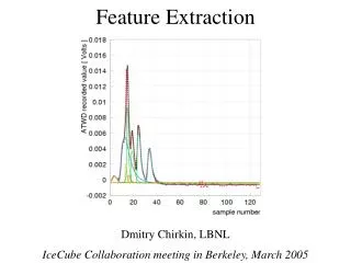
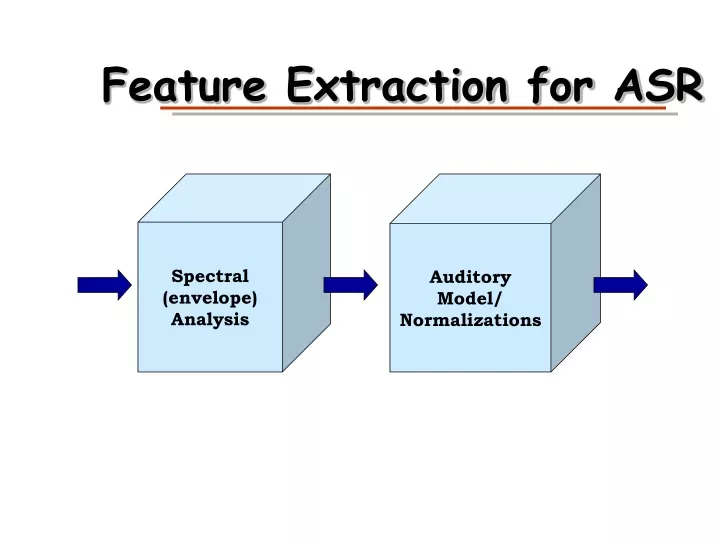
Feature Extraction for ASR. Spectral (envelope) Analysis. Auditory Model/ Normalizations. Deriving the envelope (or the excitation). excitation. Time-varying filter. h t (n). e(n). y(n)=e(n)*h t (n). HOW CAN WE GET e(n) OR h(n) from y(n)?. But first, why?.

E N D
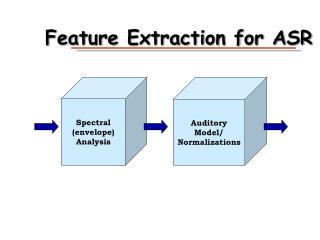
Feature Extraction for ASR Spectral (envelope)Analysis AuditoryModel/Normalizations
Deriving the envelope (or the excitation) excitation Time-varying filter ht(n) e(n) y(n)=e(n)*ht(n) HOW CAN WE GET e(n) OR h(n) from y(n)?
But first, why? • Excitation/pitch: for vocoding; for synthesis; for signal transformation; for prosody extraction (emotion, sentence end, ASR for tonal languages …); for voicing category in ASR • Filter (envelope): for vocoding; for synthesis; for phonetically relevant information for ASR
Spectral Envelope Estimation • Filters • Cepstral Deconvolution (Homomorphic filtering) • LPC
Channel vocoder (analysis) Broad w.r.t harmonics e(n)*h(n)
Bandpass power estimation B C A Rectifier Band-pass filter Low-pass filter A B C
Deriving spectral envelope with a filter bank BP 1 rectify LP 1 decimate BP 2 rectify LP 2 decimate Magnitude signals speech BP N rectify decimate LP N
Filterbank properties • Original Dudley Voder/Vocoder: 10 filters, 300 Hz bandwidth (based on # fingers!) • A decade later, Vaderson used 30 filters, • 100 Hz bandwidth (better) • Using variable frequency resolution, can use16 filters with the same quality
Mel filterbank • Warping function B(f) = 1125 ln (1 + f/700) • Based on listening experiments with pitch
Towards other deconvolution methods • Filters seem biologically plausible • Other operations could potentially separate excitation from filter • Periodic source provides harmonics (close together in frequency) • Filter provides broad influence (envelope) on harmonic series • Can we use these facts to separate?
“Homomorphic” processing • Linear processing is well-behaved • Some simple nonlinearities also permit simple processing, interpretation • Logarithm a good example; multiplicative effects become additive • Sometimes in additive domain, parts more separable • Famous example: blind deconvolution of Caruso recordings
IEEE Oral History Transcripts: Oppenheim on Stockham’s Deconvolution of Caruso Recordings (1) Oppenheim: Then all speech compression systems and many speech recognition systems are oriented toward doing this deconvolution, then processing things separately, and then going on from there. A very different application of homomorphic deconvolution was something that Tom Stockham did. He started it at Lincoln and continued it at the University of Utah. It has become very famous, actually. It involves using homomorphic deconvolution to restore old Caruso recordings. Goldstein: I have heard about that. Oppenheim: Yes. So you know that's become one of the well-known applications of deconvolution for speech. … Oppenheim: What happens in a recording like Caruso's is that he was singing into a horn that to make the recording. The recording horn has an impulse response, and that distorts the effect of his voice, my talking like this. [cupping his hands around his mouth] Goldstein: Okay.
IEEE Oral History Transcripts (2) Oppenheim: So there is a reverberant quality to it. Now what you want to do is deconvolve that out, because what you hear when I do this [cupping his hands around his mouth] is the convolution of what I'm saying and the impulse response of this horn. Now you could say, "Well why don't you go off and measure it. Just get one of those old horns, measure its impulse response, and then you can do the deconvolution." The problem is that the characteristics of those horns changed with temperature, and they changed with the way they were turned up each time. So you've got to estimate that from the music itself. That led to a whole notion which I believe Tom launched, which is the concept of blind deconvolution. In other words, being able to estimate from the signal that you've got the convolutional piece that you want to get rid of. Tom did that using some of the techniques of homomorphic filtering. Tom and a student of his at Utah named Neil Miller did some further work. After the deconvolution, what happens is you apply some high pass filtering to the recording. That's what it ends up doing. What that does is amplify some of the noise that's on the recording. Tom and Neil knew Caruso's singing. You can use the homomorphic vocoder that I developed to analyze the singing and then resynthesize it. When you resynthesize it you can do so without the noise. They did that, and of course what happens is not only do you get rid of the noise but you get rid of the orchestra. That's actually become a very fun demo which I still play in my class. This was done twenty years ago, but it's still pretty dramatic. You hear Caruso singing with the orchestra, then you can hear the enhanced version after the blind deconvolution, and then you can also hear the result after you get rid of the orchestra,. Getting rid of the orchestra is something you can't do with linear filtering. It has to be a nonlinear technique.
Log processing • Suppose y(n) = e(n)*h(n) • Then Y(f) = E(f)H(f) • And logY(f) = log E(f) + log H(f) • In some cases, these pieces are separable by a linear filter • If all you want is H, processing can smooth Y(f)
Source-filter separation by cepstral analysis Excitation Pitch detection Windowed speech Time separation Log magnitude Spectral function FFT FFT
Cepstral features • Typically truncated (smoothing) • Corresponds to spectral envelope estimation • Features also are roughly orthogonal • Common transformation for many spectral features, e.g., - filter bank energies - FFT power - LPC coefficients • Used almost universally for ASR (in some form)
Key Processing Step for ASR:Cepstral Mean Subtraction • Imagine a fixed filter h(n), so y(n)=h(n)*x(n) • Same arguments as before, but - let x vary over time - let h be fixed over time • Then average cepstra should represent the fixed component (including fixed part of x) • (Think about it)
An alternative: Incorporate Production • Assume simple excitation/vocal tract model • Assume cascaded resonators for vocal tractfrequency response (envelope) • Find resonator parameters for best spectralapproximation
= = = r2
Some LPC Issues • Error criterion • Model order
LPC Peak Modeling • Total error constrained to be (at best)gain factor squared • Error where model spectrum is largercontributes less • Model spectrum tends to “hug” peaks
More effects of error criterion • Globally tracks, but worse match inlog spectrum for low values • “Attempts” to model anti-aliasingfilter, mic response • Ill-conditioned for wide-ranging spectralvalues
Other LPC properties • Behavior in noise • Sharpness of peaks • Speaker dependence
Model Order • Too few, can’t represent formants • Too many, model detail, especially harmonics • Too many, low error, ill-conditioned matrices
Optimal Model Order • Akaike Information Criterion (AIC) • Cross-validation (trial and error)
Coefficient Estimation • Minimize squared error - set derivs to zero • Compute in blocks or on-line • For blocks, use autocorrelation or covariance methods (pertains to windowing, edge effects)
Solving the Equations • Autocorrelation method: Levinson or Durbin recursions, O(P2) ops; uses Toeplitz property (constant along left-right diagonals), guaranteed stable • Covariance method: Cholesky decomposition, • O(P3) ops; just uses symmetry property, not guaranteed stable
LPC-based representations • Predictor polynomial - ai, 1<=i<=p , direct computation • Root pairs - roots of polynomial, complex pairs • Reflection coefficients - recursion; interpolated values always stable (also called PARCOR coefficients ki, 1<=i<=p) • Log area ratios = ln((1-k)/(1+k)) , low spectral sensitivity • Line spectral frequencies - freq. pts around resonance; low spectral sensitivity, stable • Cepstra - can be unstable, but useful for recognition
Autocorrelation Analysis
Spectral Estimation CepstralAnalysis Filter Banks LPC X X X Reduced Pitch Effects X X Excitation Estimate X Direct Access to Spectra X Less Resolution at HF X Orthogonal Outputs X Peak-hugging Property X Reduced Computation