Download
1 / 30
300 likes | 439 Vues
Social Science Reasoning Using Statistics. Psychology 138 2013. Exam 2 is Wed. March 6 th Quiz 4 I will move the due date to Mon March 4 th Covers z-scores, Normal distribution, and describing correlations. Announcements. Transformations: z-scores Normal Distribution

E N D
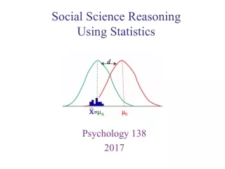
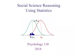
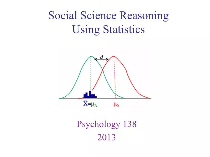
Social Science Reasoning Using Statistics Psychology 138 2013
Exam 2 is Wed. March 6th • Quiz 4 • I will move the due date to Mon March 4th • Covers z-scores, Normal distribution, and describing correlations Announcements
Transformations: z-scores • Normal Distribution • Using Unit Normal Table • Combines 2 topics Today Start the quincnux machine Outline
Number of heads HHH 3 HHT 2 HTH 2 HTT 1 THH 2 THT 1 TTH 1 TTT 0 Flipping a coin example
.4 .3 probability .2 .1 .125 .375 .375 .125 0 1 2 3 Number of heads Number of heads 3 2 2 1 2 1 1 0 Flipping a coin example
What’s the probability of flipping three heads in a row? .4 .3 probability .2 p = 0.125 .1 .125 .375 .375 .125 Think about the area under the curve as reflecting the proportion/probability of a particular outcome 0 1 2 3 Number of heads Flipping a coin example
What’s the probability of flipping at least two heads in three tosses? .4 .3 probability .2 p = 0.375 + 0.125 = 0.50 .1 .125 .375 .375 .125 0 1 2 3 Number of heads Flipping a coin example
What’s the probability of flipping all heads or all tails in three tosses? .4 .3 probability .2 p = 0.125 + 0.125 = 0.25 .1 .125 .375 .375 .125 0 1 2 3 Number of heads Flipping a coin example
Theoretical distribution (The “Bell Curve”) • Defined by density function (area under curve) for variable X given μ & σ2 • Symmetrical & unimodal; Mean = median = mode • ±1 σ are inflection points of curve (change of direction) • Common approximate empirical distribution for deviations around a continually scaled variable (errors of measurement) f(x; μ, σ2) = p asymptote z Check out the quincnux machine Normal Distribution
Use calculus to find areas under curve (rather than frequency of a score) • %(μ to 1σ) + %(μ to -1σ) ≈ 68% • p(μ < X < 1σ) + p(μ > X > -1σ) ≈ .68 • %(1σ to 2σ) + %(-1σ to -2σ) ≈ 27%, cumulative ≈ 95% (= 68%+27%) • p(1σ < X < 2σ) + p(-1σ > X > -2σ) = 27%, cumulative = .95 • %(2σ to ∞) + %(-2σ to ∞) ≈ 5%, cumulative = 100% • p(X > 2σ) + p(X < -2σ) ≈ 5%, cumulative = 1.00 100% 95% • We will use a table rather to find the probabilities rather than do the calculus. 68% p z Normal Distribution
Use known information about theoretical distributions for inferences about empirical distributions • Common approximate empirical distribution for deviations around a continually scaled variable (errors of measurement) • Decide to set p < .05 as criterion of unlikely outcomes • 2.25% score higher if z = 1.96, and 2.25% score lower if z = -1.96 • p(|z| > 1.96) = 0.05 (both tails) 2.25% 95% 2.25% Normal Distribution
Use known information about theoretical distributions for inferences about empirical distributions • Run experiment and get sample mean within 1 SD • -1 SD < M < 1 SD • How likely to get mean if draw sample randomly? • p = .68 • Was experimental intervention effective? • Probably not, too high a chance that the difference was due to random chance -1.0 1.0 68% X Normal Distribution
Use known information about theoretical distributions for inferences about empirical distributions • Run experiment and get sample mean beyond 2 SD • -1.96 SD > M > 1.96 SD • How likely to get mean if draw sample randomly? • p < .05 • Was experimental intervention effective? • Probably, very low chance that the difference was due to random chance -1.96 1.96 2.5% 2.5% X Normal Distribution
Proportions beyondz-scores • Same p-values for+ and - z-scores • p-values = 0.50 to 0.0013 z p For z = 1.00 , 15.87% beyond, p(z > 1.00) = 0.1587 1.01, 15.62% beyond, p(z > 1.00) = 0.1562 As z increases, what happens to p? p decreases Note. : indicates skipped rows Unit Normal Table, version 1(in PIP packet)
Proportions beyondz-scores • Same p-values for+ and - z-scores • p-values = 0.50 to 0.0013 For z = -1.00 , 15.87% beyond, p(z < -1.00) = 0.1587 Note. : indicates skipped rows Unit Normal Table, version 1(in PIP packet)
Proportions beyondz-scores • Same p-values for+ and - z-scores • p-values = 0.50 to 0.0013 For z = 2.00, 2.28% beyond, p(z > 2.00) = 0.0228 2.01, 2.22% beyond, p(z > 2.01) = 0.0222 As z increases, p decreases Note. : indicates skipped rows Unit Normal Table, version 1(in PIP packet)
Proportions beyondz-scores • Same p-values for+ and - z-scores • p-values = 0.50 to 0.0013 For z = -2.00, 2.28% beyond, p(z < -2.00) = 0.0228 Note. : indicates skipped rows Unit Normal Table, version 1(in PIP packet)
Proportions left of z-scores: cumulative • Requires table twice as long • p-values 0.0003 to 0.9997 50% + 34.13 = 84.13% to the left Cumulative % of population starting with the lowest value For z = +1, Unit Normal Table, cumulative version (in some other books)
Lots of places to get the Normal table • Unit normal table in your PIP packet • And online: http://psychology.illinoisstate.edu/psy138/resources/TABLES.HTMl#ztable • “Area Under Normal Curve” Excel tool (created by Dr. Joel Schneider) • Normal Density curve applet (from a textbook I used to use). This one is in today’s lab • Do a search on “Normal Table” in Google. • But be aware that there are many ways to organize the table, it is important to understand the table that you use Resources and tools
Example 1 Suppose you got 630 on SAT. What % who take SAT get your score or better? 9.68% above this score • Population parameters of SAT: μ = 500, σ = 100, normally distributed • From table: • z(1.3) =.0968 • Solve for z-value of 630. • Find proportion of normal distribution above that value. SAT examples
Example 2 Suppose you got 630 on SAT. What % who take SAT get your score or worse? 100% - 9.68% = 90.32% below score (percentile) • Population parameters of SAT: μ = 500, σ = 100, normally distributed • From table: • z(1.3) =.0968 • Solve for z-value of 630. • Find proportion of normal distribution below that value. SAT examples
In lab • Using the normal distribution • Questions? Wrap up
p beyond value p < 520 p < 450 p > 710 = 0.224 NORMDIST(B2,$B$11,$B$14,TRUE) Normal Cumulative p-value in Excel (only for normal distributions)
INVDIST(E2,$B$11,$B$14) Raw Score Given Normal Cumulative p-value in Excel (only for normal distributions)
Results from previous class Grades expressed as percentages withdrew
Sorted cases. APA Grades: SPSS Analysis
Cleaned data: 2 scores omitted. Note: SPSS SD uses sample formula. The other mode is 80. APA Grades: SPSS Analysis
APA Grades: SPSS Analysis Note how sample deviates from normal distribution. If make inferences about population of grades, get some error 108 (z = 3)
APA Grades: SPSS Analysis Skewness = -1.76 Outlier to left (discontinuous) Empty on right (truncated) Kurtosis = 6.05 Leptokurtic (narrow, peaked, leaping) Platykurtic (broad, flat, platypus) Mesokurtic (normal)