Download
1 / 19
190 likes | 303 Vues
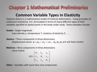
Chapter 1 Mathematical Preliminaries. Common Variable Types in Elasticity.

E N D
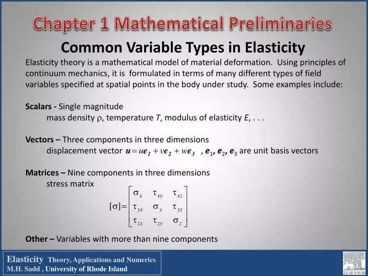
Chapter 1 Mathematical Preliminaries Common Variable Types in Elasticity Elasticity theory is a mathematical model of material deformation. Using principles of continuum mechanics, it is formulated in terms of many different types of field variables specified at spatial points in the body under study. Some examples include: Scalars - Single magnitude mass density , temperature T, modulus of elasticity E, . . . Vectors – Three components in three dimensions displacement vector Matrices – Nine components in three dimensions stress matrix Other – Variables with more than nine components , e1, e2, e3 are unit basis vectors ElasticityTheory, Applications and NumericsM.H. Sadd , University of Rhode Island
Index/Tensor Notation With the wide variety of variables, elasticity formulation makes use of a tensor formalism using index notation. This enables efficient representation of all variables and governing equations using a single standardized method. Index notation is a shorthand scheme whereby a whole set of numbers or components can be represented by a single symbol with subscripts In general a symbol aij…k with N distinct indices represents 3N distinct numbers Addition, subtraction, multiplication and equality of index symbols are defined in the normal fashion; e.g. ElasticityTheory, Applications and NumericsM.H. Sadd , University of Rhode Island
Notation Rules and Definitions Summation Convention - if a subscript appears twice in the same term, summation over that subscript from one to three is implied; for example A symbol aij…m…n…k is said to be symmetric with respect to index pair mn if A symbol aij…m…n…k is said to be antisymmetricwith respect to index pair mn if Useful Identity . . . antisymmetric . . . symmetric ElasticityTheory, Applications and NumericsM.H. Sadd , University of Rhode Island
Example 1-1: Index Notation Examples The matrix aij and vector biare specified by Determine the following quantities: Indicate whether they are a scalar, vector or matrix. Following the standard definitions given in section 1.2, ElasticityTheory, Applications and NumericsM.H. Sadd , University of Rhode Island
Special Index Symbols KroneckerDelta Properties: Alternating or Permutation Symbol 123 = 231 = 312 = 1, 321 = 132 = 213 = -1, 112 = 131 = 222 = . . . = 0 Useful in evaluating determinants and vector cross-products ElasticityTheory, Applications and NumericsM.H. Sadd , University of Rhode Island
x3 x3 v x2 e3 e3 e2 x2 e2 e1 e1 x1 x1 Coordinate Transformations To express elasticity variables in different coordinate systems requires development of transformation rules for scalar, vector, matrix and higher order variables – a concept connected with basic definitions of tensor variables. The two Cartesian frames (x1,x2,x3) and differ only by orientation Using Rotation Matrix transformation laws for Cartesian vector components ElasticityTheory, Applications and NumericsM.H. Sadd , University of Rhode Island
Cartesian TensorsGeneral Transformation Laws Scalars, vectors, matrices, and higher order quantities can be represented by an index notational scheme, and thus all quantities may then be referred to as tensors of different orders. The transformation properties of a vector can be used to establish the general transformation properties of these tensors. Restricting the transformations to those only between Cartesian coordinate systems, the general set of transformation relations for various orders are: ElasticityTheory, Applications and NumericsM.H. Sadd , University of Rhode Island
x3 x3 x2 x2 60o x1 x1 Example 1-2 Transformation Examples The components of a first and second order tensor in a particular coordinate frame are given by Determine the components of each tensor in a new coordinate system found through a rotation of 60o (/6 radians) about the x3-axis. Choose a counterclockwise rotation when viewing down the negative x3-axis, see Figure 1-2. The original and primed coordinate systems are shown in Figure 1-2. The solution starts by determining the rotation matrix for this case The transformation for the vector quantity follows from equation (1.5.1)2 and the second order tensor (matrix) transforms according to (1.5.1)3 ElasticityTheory, Applications and NumericsM.H. Sadd , University of Rhode Island
Principal Values and Directions for Symmetric Second Order Tensors The direction determined by unit vector n is said to be a principal direction or eigenvector of the symmetric second order tensor aij if there exists a parameter (principal value or eigenvalue) such that Relation is a homogeneous system of three linear algebraic equations in the unknowns n1, n2, n3. The system possesses nontrivial solution if and only if determinant of coefficient matrix vanishes scalars Ia, IIa and IIIa are called the fundamental invariants of the tensor aij ElasticityTheory, Applications and NumericsM.H. Sadd , University of Rhode Island
Principal Axes of Second Order Tensors It is always possible to identify a right-handed Cartesian coordinate system such that each axes lie along principal directions of any given symmetric second order tensor. Such axes are called the principal axes of the tensor, and the basis vectors are the principal directions {n(1), n(2) , n(3)} x3 x2 x1 Original Given Axes Principal Axes ElasticityTheory, Applications and NumericsM.H. Sadd , University of Rhode Island
Example 1-3 Principal Value Problem Determine the invariants, and principal values and directions of First determine the principal invariants The characteristic equation then becomes Thus for this case all principal values are distinct For the 1 = 5 root, equation (1.6.1) gives the system which gives a normalized solution In similar fashion the other two principal directions are found to be It is easily verified that these directions are mutually orthogonal. Note for this case, the transformation matrix Qij defined by (1.4.1) becomes ElasticityTheory, Applications and NumericsM.H. Sadd , University of Rhode Island
Vector, Matrix and Tensor Algebra Scalar or Dot Product Vector or Cross Product Common Matrix Products ElasticityTheory, Applications and NumericsM.H. Sadd , University of Rhode Island
Calculus of Cartesian Tensors Field concept for tensor components Comma notationfor partial differentiation If differentiation index is distinct, order of the tensor will be increased by one; e.g. derivative operation on a vector produces a second order tensor or matrix ElasticityTheory, Applications and NumericsM.H. Sadd , University of Rhode Island
Vector Differential Operations Directional Derivative of Scalar Field Common Differential Operations ElasticityTheory, Applications and NumericsM.H. Sadd , University of Rhode Island
Example 1-4: Scalar/Vector Field Example Scalar and vector field functions are given by Calculate the following expressions, , 2, ∙ u, u, u. Contours =constant and vector distributions of vector field is orthogonal to -contours (ture in general ) Using the basic relations: 2 - (satisfies Laplace equation) ∙ u u u y x ElasticityTheory, Applications and NumericsM.H. Sadd , University of Rhode Island
Vector/Tensor Integral Calculus Divergence Theorem Stokes Theorem Green’s Theorem in the Plane Zero-Value Theorem ElasticityTheory, Applications and NumericsM.H. Sadd , University of Rhode Island
Orthogonal Curvilinear Coordinate Systems x3 e3 R x2 e2 e1 x1 Spherical Coordinate System (R,,) Cylindrical Coordinate System (r,,z) ElasticityTheory, Applications and NumericsM.H. Sadd , University of Rhode Island
General Curvilinear Coordinate Systems Common Differential Forms ElasticityTheory, Applications and NumericsM.H. Sadd , University of Rhode Island
Example 1-5: Polar Coordinates From relations (1.9.5) or simply using the geometry shown in Figure The basic vector differential operations then follow to be ElasticityTheory, Applications and NumericsM.H. Sadd , University of Rhode Island