Download
1 / 56
580 likes | 752 Vues
Computer Simulation of Geologic Sequestration of CO 2. PhD Defense Akand W. Islam Department of Chemical and Biological Engineering The University of Alabama Adviser: Dr. Eric S. Carlson. 10/17/2012.

E N D
Computer Simulation of Geologic Sequestration of CO2 PhD Defense Akand W. Islam Department of Chemical and Biological Engineering The University of Alabama Adviser: Dr. Eric S. Carlson 10/17/2012
1. A Fully Non-iterative Technique for Phase Equilibrium and Density Calculations of CO2+Brine System and an Equation of State for CO2 Objective The objective of this research is to develop a fully non-iterative algorithm for phase equilibrium and density calculations of CO2+Brine system for efficient numerical simulations of CO2 flows. Proceedings of the 37th Stanford Geothermal Workshop, Stanford University, 2012.
1.Phase Equilibrium and Density Calculations of CO2+Brine Inputs: • P (system pressure) • T (system temperature) • mNaCl (molality of NaCl) Equation to be solved: Proceedings of the 37th Stanford Geothermal Workshop, Stanford University, 2012.
1. Phase Equilibrium and Density Calculations of CO2+Brine Calculating volume of CO2: • Solving V = V(V,P,T) [From Redlick-Kwong Equation of State] • Calculating V from V=V(P,T) ??? Proceedings of the 37th Stanford Geothermal Workshop, Stanford University, 2012.
1. Phase Equilibrium and Density Calculations of CO2+Brine Equation of State (empirical) for CO2 Where Proceedings of the 37th Stanford Geothermal Workshop, Stanford University, 2012.
1. Phase Equilibrium and Density Calculations of CO2+Brine Equation of state for CO2: (validation) Proceedings of the 37th Stanford Geothermal Workshop, Stanford University, 2012.
1. Phase Equilibrium and Density Calculations of CO2+Brine Results Proceedings of the 37th Stanford Geothermal Workshop, Stanford University, 2012.
1. Phase Equilibrium and Density Calculations of CO2+Brine Results Proceedings of the 37th Stanford Geothermal Workshop, Stanford University, 2012.
1. Phase Equilibrium and Density Calculations of CO2+Brine Results Proceedings of the 37th Stanford Geothermal Workshop, Stanford University, 2012.
1. Phase Equilibrium and Density Calculations of CO2+Brine Comparisons of computations time *3 GB Ram, Dual-core CPU T4500 @ 2.3 GHz **11.57 GB, i7-920 CPU @ 2.67 GHz Proceedings of the 37th Stanford Geothermal Workshop, Stanford University, 2012.
1. Phase Equilibrium and Density Calculations of CO2+Brine Advantages: • Complete mathematical non-iterative tool for calculation of phase equilibrium and density. • Calculate the data within 1% deviation • High pressure range (1-400 bar) • Computationally very efficient Limitation: • Small temperature range (20-40 °C) for phase equilibrium computation Proceedings of the 37th Stanford Geothermal Workshop, Stanford University, 2012.
2. Modification of Liquid State Models for the Phase Equilibrium Calculations of Supercritical CO2 and H2O at High Temperatures and Pressures Objective The objective of this work is to modify the liquid state models by introducing pressure and temperature dependent terms and then predict the appropriate parameters which can regenerate the literature CO2 and H2O solubility data within fair deviation. Geothermal Resources Council Trans., 36, 855-861, 2012
2. Liquid State Models Inputs: • P (system pressure) • T (system temperature) • Zi (feed composition) Equation to be solved: Geothermal Resources Council Trans., 36, 855-861, 2012
2. Liquid State Models Two-parameter Models: • UNIQUAC • LSG Three-parameter Models: • NRTL • GEM-RS Geothermal Resources Council Trans., 36, 855-861, 2012
2. Liquid State Models (binary interaction parameters) Two-parameter Models: • UNIQUAC • LSG Three-parameter Models: • NRTL • GEM-RS Geothermal Resources Council Trans., 36, 855-861, 2012
2. Liquid State Models (modification of interaction parameters) Two-parameter Models: • UNIQUAC • LSG Three-parameter Models: • NRTL • GEM-RS Geothermal Resources Council Trans., 36, 855-861, 2012
2. Liquid State Models (Results) **AAE (average absolute error) = [k = 1 (solubility of CO2 in water), and k = 2 (solubility of H2O in CO2)] whereN=NK*Ni Geothermal Resources Council Trans., 36, 855-861, 2012
2. Liquid State Models (Results) Geothermal Resources Council Trans., 36, 855-861, 2012
2. Liquid State Models (comparative results) Geothermal Resources Council Trans., 36, 855-861, 2012
2. Liquid State Models Comparisons of computations time Geothermal Resources Council Trans., 36, 855-861, 2012
2. Liquid State Models Advantages: • No Equation of State • No mixing rule • No complexity for computing fugacity coefficient • Only flash type algorithm Limitation: • applicable only at high temperatures and pressures • No density measurement, only phase compositions Geothermal Resources Council Trans., 36, 855-861, 2012
3. Application of SAFT equation for CO2+H2O phase equilibrium calculations over a wide temperature and pressure range Objective: To employ the statistical associating fluid theory (SAFT) equation of state for the correlation and prediction of vapor – liquid equilibrium of CO2+H2O binary system for a wide temperature (10 – 300 °C) and pressure (1 – 600 bar) ranges. Fluid Phase Equilibria, 321, 17-24, 2012.
3. SAFT Equation of State Here is the free energy of hard-sphere fluid; is the free energy associated with the formation of chains from hard spheres; and are the contributions to the free energy of dispersion and association interactions, respectively. Fluid Phase Equilibria, 321, 17-24, 2012.
3. SAFT Equation of State The effective number of segments, mi The energy parameter of the L-J (Lennard-Jones), Fluid Phase Equilibria, 321, 17-24, 2012.
3. SAFT Equation of State (Results) Fluid Phase Equilibria, 321, 17-24, 2012.
3. SAFT Equation of State (Results) Fluid Phase Equilibria, 321, 17-24, 2012.
3. SAFT Equation of State (Results) Fluid Phase Equilibria, 321, 17-24, 2012.
3. SAFT Equation of State (Results) Fluid Phase Equilibria, 321, 17-24, 2012.
3. SAFT Equation of State Advantages: • Theoretically sound • Compute the data with less than 2% deviation • Very wide temperature and pressure range Limitation: • Complex equation and thus computationally not much efficient Fluid Phase Equilibria, 321, 17-24, 2012.
4. Viscosity models and effects of dissolved CO2 Objective The objective of this work is to study one of the transport properties, viscosity, and present some simpler and more efficient tools to compute the viscosity of pure water, H2O+CO2, brine (H2O+NaCl and H2O+NaCl+CO2), and typical seawater (3.5% salinity) for the pressure and temperature range of 1-600 bar and 20-105 °C, respectively. In addition, how viscosity varies quantitatively for CO2 dissolution in the aqueous phase is analyzed. Energy & Fuels, 26, 5330-5336, 2012.
4. Viscosity models and effects of dissolved CO2 Viscosity of pure H2O: Energy & Fuels, 26, 5330-5336, 2012.
4. Viscosity models and effects of dissolved CO2 Viscosity of pure H2O (comparisons): Energy & Fuels, 26, 5330-5336, 2012.
4. Viscosity models and effects of dissolved CO2 Viscosity of H2O+NaCl: where, Energy & Fuels, 26, 5330-5336, 2012.
4. Viscosity models and effects of dissolved CO2 Viscosity of H2O+NaCl: Energy & Fuels, 26, 5330-5336, 2012.
4. Viscosity models and effects of dissolved CO2 Viscosity of H2O+CO2: where, Energy & Fuels, 26, 5330-5336, 2012.
4. Viscosity models and effects of dissolved CO2 Viscosity of H2O+CO2: Energy & Fuels, 26, 5330-5336, 2012.
4. Viscosity models and effects of dissolved CO2 Viscosity of H2O+NaCl+CO2: Energy & Fuels, 26, 5330-5336, 2012.
4. Viscosity models and effects of dissolved CO2 Viscosity of H2O+NaCl+CO2: Energy & Fuels, 26, 5330-5336, 2012.
4. Viscosity models and effects of dissolved CO2 Viscosity of Saline water: Energy & Fuels, 26, 5330-5336, 2012.
4. Viscosity models and effects of dissolved CO2 Effects of dissolved CO2 Energy & Fuels, 26, 5330-5336, 2012.
4. Viscosity models and effects of dissolved CO2 Conclusions • At lower temperatures (<40 °C) the effect of CO2 dissolution is large, specially at saturated condition. • At 20 °C and 50 bar, viscosity of water with saturated CO2 is ~21% higher than with no CO2. At 600 bar this is ~38%. • Neglecting CO2’s presence in brine also warrant error. • At 20 °C, and at 50 and 600 bar, CO2 saturation in brine (1 molal) contributes viscosity increase by 16% and 22%, respectively, higher. • After 50 °C, effects of dissolved CO2 decrease. Energy & Fuels, 26, 5330-5336, 2012.
5. Double diffusive natural convection of CO2 in porous media Model Geothermics (in review)
5. Double diffusive natural convection of CO2 in porous media Governing Equations (5.1) (5.2) Stream function (5.3) Concentration equation (5.4) Energy equation Here, Geothermics (in review)
5. Double diffusive natural convection of CO2 in porous media Investigations Solutal Rayleigh no., Ras = 100, 1000, 10000 Bouyancy Ratio, N = -100, -10, -2 Reservoir shape, A = 0.5,1, 2 Geothermics (in review)
5. Double diffusive natural convection of CO2 in porous media Results t = 500 yrs t = 500 yrs Ras = 100, N = 100, A = 1 Ras = 1000, N = 100, A = 1 Geothermics (in review)
5. Double diffusive natural convection of CO2 in porous media t = 68 yrs Results t = 4 yrs t = 100 yrs t = 10 yrs t = 500 yrs t = 20 yrs Geothermics (in review) Ras = 10000, N = 100, A = 1
5. Double diffusive natural convection of CO2 in porous media Results t = 100 yrs t = 4 yrs t = 500 yrs t = 20 yrs Ras = 10000, N = 2, A = 1 Geothermics (in review)
5. Double diffusive natural convection of CO2 in porous media Results t = 500 yrs t = 500 yrs N = 2 N = 100 Ras = 10000, A = 0.5 Geothermics (in review)
5. Double diffusive natural convection of CO2 in porous media Results t = 500 yrs t = 500 yrs N = 2 N = 100 Ras = 10000, A = 2 Geothermics (in review)
5. Double diffusive natural convection of CO2 in porous media Results Geothermics (in review) A = 1