Download
1 / 11
110 likes | 203 Vues
Frequency dependent Measurement and theoretical Prediction of Characteristic Parameters of Vacuum Cable Micro-Striplines. - Risetime of a typical ATLAS LAr pulse is approx. 20 ns, corresponding to a bandwidth of 17.5 MHz. - Explore the frequency dependent behaviour of the vacuum cable

E N D
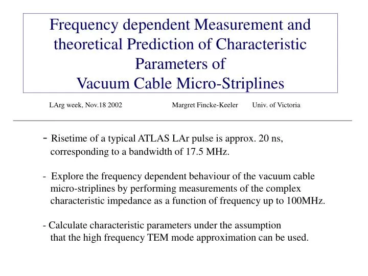
Frequency dependent Measurement and theoretical Prediction of Characteristic Parameters ofVacuum Cable Micro-Striplines - Risetime of a typical ATLAS LAr pulse is approx. 20 ns, corresponding to a bandwidth of 17.5 MHz. - Explore the frequency dependent behaviour of the vacuum cable micro-striplines by performing measurements of the complex characteristic impedance as a function of frequency up to 100MHz. - Calculate characteristic parameters under the assumption that the high frequency TEM mode approximation can be used. LArg week, Nov.18 2002 Margret Fincke-Keeler Univ. of Victoria
Measure: magnitude and phase of the stripline impedance for open circuit and short circuit termination: g complex impedances Zoc , Zsc Calculate the complex characteristic impedance: And the quantity: With: l = length of stripline, g = propagation coeff. = a + ib a = attenuation coeff. b = phase change coeff. M. Fincke-Keeler Univ. of Victoria
Impedance and attenuation coefficient 50 Zo [Ω] 40 30 20 5 10 15 20 25 30 35 40 45 frequency [MHz] 0.14 0.10 atten. coeff α 0.06 0.02 5 10 15 20 25 30 35 40 45 frequency [MHz] M. Fincke-Keeler Univ. of Victoria
Calculate: Resistance Inductance Conductance Capacitance Phase velocity: Dielectric constant: M. Fincke-Keeler Univ. of Victoria
Primary transmission line parameters: R, L, G, C 10 20 30 40 frequency[MHz] 10 20 30 40 frequency[MHz] 10 20 30 40 frequency[MHz] 10 20 30 40 frequency[MHz]
Phase velocity and relative dielectric constant p 5 10 15 20 25 30 35 40 45 frequency [MHz] 5 10 15 20 25 30 35 40 45 frequency [MHz] M. Fincke-Keeler Univ. of Victoria
Theoretical description For a given strip line geometry, solve Laplace’s equation numerically to obtain the capacitance per unit length. 1V Do the calculation twice: once with εr=0 around the copper strips (vacuum) once with εr for polyimide and adhesive materials. Obtain: capacitance of Cu strips in vacuum Cv capacitance of Cu strips in dielectric Cε =w M. Fincke-Keeler Univ. of Victoria
strip thick- ness εr Poly- imide εr adhe- sive signal width ground width Cυ Cε Zo f M. Fincke-Keeler Univ. of Victoria
Now we can calculate: We can determine R from the resistivity of copper and the cross sectional area of the copper strips. The skin effect has been taken into account in a simplified approximation. Now we can calculate: and it follows: where loc , lscare the electrical lengths of the stripline with open circuit and Short cuircuit termination respectively. M. Fincke-Keeler Univ. of Victoria
Comparison between measurement and theoretical Prediction. Signal Width = 190μm Ground width = 360μm Thickness = 34μm εr (polyimide)=3.2 εr (adhesive)=4.0 20 40 60 80 frequency[MHz] 20 40 60 80 frequency[MHz] 20 40 60 80 frequency[MHz] 20 40 60 80 frequency[MHz] M. Fincke-Keeler Univ. of Victoria
Conclusions • - The complex characteristic impedance of the vacuum cable • micro-striplines has been measured as a function of frequency. • A numerical solution of Laplace’s equation yields the values • of the capacitances Cυ and Cε of the copper strips in vacuum • and in dielectric respectively, and allows the calculation of • the characteristic line parameters for that geometry. • The results of the theoretical calculations are in good agreement • with the measurement. • The differences between the calculation and data are most • likely due to the approximation and assumptions made for • the calculations (e.g. high freq. TEM mode, skin effect). M. Fincke-Keeler Univ. of Victoria