Download
1 / 26
260 likes | 342 Vues
Using the Maryland Biological Stream Survey Data to Test Spatial Statistical Models. N. Scott Urquhart Joint work with Erin P. Peterson, Andrew A. Merton, David M. Theobald, and Jennifer A. Hoeting All of Colorado State University, Fort Collins, CO 80523-1877. This research is funded by

E N D
Using the Maryland Biological Stream Survey Data to Test Spatial Statistical Models N. Scott Urquhart Joint work with Erin P. Peterson, Andrew A. Merton, David M. Theobald, and Jennifer A. Hoeting All of Colorado State University, Fort Collins, CO 80523-1877
This research is funded by U.S.EPA – Science To Achieve Results (STAR) Program Cooperative Agreement # CR - 829095 FUNDING ACKNOWLEDGEMENT The work reported here today was developed under the STAR Research Assistance Agreement CR-829095 awarded by the U.S. Environmental Protection Agency (EPA) to Colorado State University. This presentation has not been formally reviewed by EPA. The views expressed here are solely those of presenter and STARMAP, the Program he represents. EPA does not endorse any products or commercial services mentioned in this presentation.
Expected Results: • A geostatistical model • Predict a specific reach scale condition at points that were not sampled • Provide a better understanding of the relationship between the landscape and reach scale conditions • Give insight into potential sources of water quality degradation • Develop landscape indicators • Crucial for the rapid and cost efficient monitoring of large areas • Better understanding of spatial autocorrelation in stream networks • What is the distance within which it occurs? • How does that differ between chemical variables? • Products: • Map of the study area • Shows the likelihood of water quality impairment for each stream segment • Based on water quality standards or relative condition (low, medium, high) • Future sampling efforts can be concentrated in areas with a higher probability of impairment • Methodology • Illustrates how States and Tribes can complete spatial analysis using GIS data and field data • GIS tools will be available
OUR PATH TODAY • What are “Spatial Statistical Models”? • Measuring Distance in Space • The Maryland Biological Stream Survey • Outstanding data set to compare models • A Few Results • Work in Progress
GATHERING SOME INSIGHTS • Raise your hand if you • Had a statistics course – even in the distant past • Remember doing a t-test • Did a simple linear regression (fitted a line) • Did a multiple regression • Examined model failures • Did analyses accommodating “correlated errors” • Have used spatial statistics, eg, kreiging
STATISTICS AND PREDICTION • OBJECTIVE: Measure relevant responses, • Like dissolved organic carbon (DOC), and • Related variables at suitable sites, then • Develop formula to predict DOC at • Unvisited sites • Why? • Clean Water Act (CWA) 303(d) • requires states to identify “impacted” waters and plan to eliminate impact • What state has the $ to evaluate every water? Predict, instead.
PREDICTIVE VARIABLES • Predict DOC from measures such as • Area above the stream evaluation point • % Barren • % High Intensity Urban • % Woody Wetland (*) • % Conifer or Evergreen Forest Type (*) • % Mixed Forest Type (*) • % low intensity Urban (*) • To accommodate year diff’s: • 1996 & 1997 (*)
GIS TOOLS • These variables require • Efficient delineation of watershed above any point • STARMAP has developed such software • It is available • Documented in a poster
PREDICTIVE MODELS • Classical regression model would be: • BUT “Everything is related to everything else, but near things are more related than distant things” Tobler (1970). • Thus the “uncorrelated” above is indefensible in many cases
SO WHAT ISSPATIAL STATISTICS? • Spatial Statistics is a set of techniques which • Allow correlated data • Index the amount of correlation by distance the points are apart • Incorporate this correlation into predictions
The Maryland Biological Stream Survey • Outstanding data set to compare models
The Clean Water Act (CWA) of 1972 requires • States, tribes, & territories to identify water quality (WQ) impaired stream segments • Create a priority ranking of those segments • Calculate the Total Maximum Daily Load (TMDL) for each impaired segment based upon chemical and physical WQ standards • A biannual inventory characterizing regional WQ • The Problem • It is impossible to physically sample every stream within a large area • Too many stream segments • Limited personnel • Cost associated with sampling • Probability-based inferences used to generate regional estimates of WQ • In miles by stream order • Does not indicate where WQ impaired segments are located • A rapid and cost-efficient method needed to locate potentially impaired stream segments throughout large areas • Our Approach • Develop a geostatistical model based on coarse-scale geographical information system (GIS) data • Make predictions for every stream segment throughout a large area • Generate a regional estimate of stream condition • Identify potentially WQ impaired stream segments • The Clean Water Act (CWA) of 1972 requires • States, tribes, & territories to identify water quality (WQ) impaired stream segments • Create a priority ranking of those segments • Calculate the Total Maximum Daily Load (TMDL) for each impaired segment based upon chemical and physical WQ standards • A biannual inventory characterizing regional WQ • The Problem • It is impossible to physically sample every stream within a large area • Too many stream segments • Limited personnel • Cost associated with sampling • Probability-based inferences used to generate regional estimates of WQ • In miles by stream order • Does not indicate where WQ impaired segments are located • A rapid and cost-efficient method needed to locate potentially impaired stream segments throughout large areas • Our Approach • Develop a geostatistical model based on coarse-scale geographical information system (GIS) data • Make predictions for every stream segment throughout a large area • Generate a regional estimate of stream condition • Identify potentially WQ impaired stream segments
Dissolved Organic Carbon (DOC) Example • Fit a geostatistical model to DOC data and coarse-scale watershed characteristics • Maryland Biological Stream Survey data 1996 • 7 interbasins & 343 DOC survey sites • GIS data:
Methods • Pre-process GIS data • “Snap” survey sites to streams • Calculate watershed attributes using the Functional Linkage of Watersheds and Streams (FLoWS) tools (Theobald et al., 2005; Peterson et al., in review) • Calculate distance matrices for model selection • R statistical software • x,y coordinates for observed survey sites • Test all possible linear models using the 10 covariates • 1024 models (210 = 1024) • Distance measure: Straight-line distance (aka Euclidean) • Autocorrelation function: Mariah • Estimate autocorrelation parameters: nugget, sill, and range • Profile-log likelihood function • Model Selection • Spatial Akaike Information Corrected Criterion (AICC) • (Hoeting et al., in press) • Mean square prediction error (MSPE)
Model Results • Range of spatial autocorrelation: 21.09 kilometers • Significant watershed attributes = WATER, EMERGWET, WOODYWET, FELPERC, and MIN TEMP • Model fit • Leave-one-out cross validation method and Universal kriging • Overall MSPE = 0.93, R2 = 0.72 • One strongly influential site • R2 without the influential site = 0.66
East-West trend in model fit • Conservative model fit: tends to underestimate DOC • 35 MSPE values > 1.5 • These sites have similar covariate values to nearby sites, but considerably different DOC values than nearby sites
Model Predictions • Create prediction sites • 1st, 2nd, and 3rd order non-tidal stream segments • 3083 prediction sites = downstream node of each GIS stream segment • Downstream node ensures that entire segment is located in same watershed • More than one prediction location at stream confluences • Covariates for prediction sites represent the conditions upstream from the segment, not the stream confluence • Calculate distance matrices for model predictions • Include observed and predicted survey sites • Generate predictions and prediction variances • Assign values back to stream segments in GIS • Universal kriging Algorithm Prediction statistics
18 prediction values > 15.9 mg/l • Also possessed 18 largest prediction variances • Located in watersheds with large WATER, EMERGWET, or WOODYWET values • Large covariate values are not represented in the observed covariate data • Represent 5973.03 kilometers of stream miles
Products • Geostatistical model used to predict segment-scale WQ conditions at unobserved locations • Map of the study area that shows the likelihood of WQ impairment for each segment • Can be tied to threshold values or WQ standards • Technical and Regulatory Services Administration within the Maryland Department of the Environment • Modifying the USGS NHD to include: • watershed impairments & stream-use designations by NHD segment • Frank Siano, personal communication • A methodology that illustrates how agencies can accomplish spatial analysis using GIS data, MBSS data, and geostatistics • The Advantages • Additional sampling is not necessary • Compliments existing methodologies • Derive a regional estimate of stream condition in two ways: • Probability-based inferences about stream miles by stream order • Sum prediction values in miles by stream order • Identify potentially WQ impaired stream segments • Methodology can be used for regulated constituents as well • Nitrate, acid neutralizing capacity, pH, and conductivity can be accurately predicted using geostatistical models (Peterson et al., in review2) • Identify spatial patterns of WQ throughout a large area • Identify areas where additional samples would provide the most information • Model results can be displayed visually • Allows professionals to communicate results with a wide variety of audiences easily
References Hoeting J.A., Davis R.A., & Merton A.A., Thompson S.E. (in press) Model Selection for Geostatistical Models. Ecological Applications. http://www.stat.colostate.edu/%7Ejah/papers/index.html Peterson E.E., Theobald D.M., & Ver Hoef J.M. (in review1) Support for geostatistical modeling on stream networks: Developing valid covariance matrices based on hydrologic distance and stream flow. Freshwater Biology. Peterson E.E., Merton A.A., Theobald D.M., & Urquhart N.S. (in review2) Patterns of Spatial Autocorrelation in Stream Water Chemistry. Environmental Monitoring. Theobald D.M., Norman J., Peterson E.E., Ferraz S. (2005) Functional Linkage of Watersheds and Streams (FLoWs) Network-based ArcGIS tools to analyze freshwater ecosystems. Proceedings of the ESRI User Conference 2005. July 26, 2005, San Diego, CA, USA. Acknowledgements The work reported here was developed under STAR Research Assistance Agreement CR-829095 awarded by the U.S. Environmental Protection Agency to the Space Time Aquatic Resource Modeling and Analysis Program (STARMAP) at Colorado State University. This poster has not been formally reviewed by the EPA. The views expressed here are solely those of the authors. The EPA does not endorse any products or commercial services presented in this poster.