Download
1 / 31
370 likes | 1.03k Vues
Spatial Statistics in Ecology: Point Pattern Analysis. Lecture Two. Re-Cap and Introduction to Point Pattern Analysis. First-order effects look at trends over space

E N D
Spatial Statistics in Ecology:Point Pattern Analysis Lecture Two
Re-Cap and Introduction to Point Pattern Analysis • First-order effects look at trends over space • Second order effects look at PAIRS OF POINTS i.e. the spatial dependence or covariance structure of pairs of variables over space • Spatial dependence gives rise to different types of processes
Types of Processes HOMOGENEOUS or stationary processes • Mean is constant over R (space) • Variance is constant over R • Covariance is dependant on DISTANCE AND DIRECTION So……………there is NO global trend! ……………….there is NO first order effect!
Types of Processes HETEROGENEOUS processes or non-stationarity • Constant mean • Constant variance • Covariance is ONLY dependant on DISTANCE SO………….your process is ISOTROPIC!
Point Patterns • Recall that point patterns deal with events that occur in discrete locations • Point patterns consist of events with variation in the mean value of the event • Can you think of what types of point patterns ecologists deal with? They will all be either: RANDOM, CLUMPED or HOMOGENEOUS
Is the distribution clustered or regular? • s1, s2, s3, s4 are “events” which have coordinates (x,y) in area “R”. • “events” are objects with various “intensity” in this case height Study region = R s1 s3 1.2m 1.8m s2 s4 1.6m 1.6m
Isotropic versus Stationary Intensity = (s) for a first-order property. For a stationary process this is constant over R. For second-order intensity = (si, sj). If its isotropic spatial dependence is a function of length = h (distance). If its stationary it depends on only vector distance (both direction and distance) not on absolute location s1 s3 isotropic 1.8m 1.2m h s2 s4 h 1.6m 1.6m stationary Study region = R
Visualizing point patterns Visualization is the simplest method to use for point pattern analysis. These are called dot maps. What would happen to the observed patterns of the scale (grain or extent) changed? – A random pattern can look ordered if the scale in too small. What type of patterns are these?
Exploring spatial point patterns Statistics and plots can be derived for point patterns. These can be used to describe the pattern or how mean values of points change across space. The simplest is the QUADRAT METHOD. The # of events per unit area are counted and divided by area of each square to get a measure of the intensity of each quadrat
Quadrat Methods This can tell is something about how the processes changes over R. We have now transformed our data into area data. There are obvious problems with this type of approach however. We throw away a lot of spatial detail and the “edge” effects may give us a different pattern to the one we observe. Doesn’t take into account relative position of points and is dependant on this size of the grid. Close points also count as much as far points!
Edge corrections should be used if points are near the edge Tao is the bandwidth and determines resolution Point A Point B Kernel Estimation Kernel estimation weights points that are further away less than those that are close. Point A will count less than Point B.
Bandwidth is important With a very large bandwidth no pattern is seen. With a very small bandwidth there is too fine a resolution to see patterns. Which bandwidth picks up the trend?
Second Order-effects • Recall that second order effects deal with PAIRS OF POINTS • How do variables covary at each point in space • Nearest-neighbor techniques are the most commonly used
Nearest-neighbor techniques 2 1 3 6 5 4 7
Distribution functions NN can be used to create an event-event plot If the slope rises fast the points are dense (ie. the pairs of NN are clustered together). This is subjective though and makes no corrections for edge effects OR for points other than the NN
Second-Order Point Pattern Analysis: The K function K(h)= E • = measure of mean intensity • = n R n= events R (area of observation) K= k function h= distance So…this tells you the expected # of events within distance h of a randomly selected event The K analysis provides a measure of the reduced second moment measure or K function of the observed process. This provides a more effective summary at a wider range of scales. However, care must be taken that within the scale of interest the data is homogeneous or isotropic.
R = 40km2 i j No events within distance h from event j N =120 = 3 (events per km2) h = 2 Corrects for the edge effect How does it work? To get the k function you visit all 120 events and find how many are within a distance of 2 km from each event. This is done for each 2 events within distance h from event i
Edge Effects Edge effects can seriously degrade distance-based statistics, and there are at least two ways to deal with these. One way is to invoke a buffer area around the study area, and to analyze only a smaller area nested within the buffer. By common convention, the analysis is restricted to distances of half the smallest dimension of the study area. This, of course, is expensive in terms of the data not used in the analysis. A second approach is to apply an edge correction to the indicator function for those points that fall near the edges of the study area; Ripley and others have suggested a variety of geometric corrections.
Confidence Limits Ripley derived approximations of the test of significance for normal data. But data are often not normal, and assumptions about normality are particularly suspect under edge effects. So in practice, the K function is generated from the test data, and then these data are randomized to generate the test of significance as confidence limits. For example, if one permuted the data 99 times and saved the smallest and largest values of L(d) for each d, these extremes would indicate the confidence limits at alpha=0.01; that is, an observed value outside these limits would be a 1-in-a-hundred chance. Likewise, 19 randomizations would yield the 95% confidence limits [Note that these estimates are actually rather imprecise; simulations suggest that it might require 1,000-5,000 randomizations to yield precise estimates of the 95% confidence limits, and >10,000 randomizations to yield precise 99% limits.]
Modelling Spatial Point Patterns: First-order -- CSR • Modelling of spatial point patterns is done using the COMPLETE SPATIAL RANDOMNESS (CSR) model. • Events follow a homogenous Poisson process over the study region (which as we know is normally violated) • CSR provides a baseline of complete randomness from which we can quantify deviations as regular or clustered
How does it work? Regularity in the first map and clustering in the second can be quantified as departures from randomness. Either event-event or point-event distances are used. This can only tell us that there is a departure from CSR. The K function can also be extended with its focus on dependence over a range of scales however if second-order effects are present (in our case there are obvious spatial effects) other methods should be used
Locations of redwood seedlings in a forest: Population Level Many spatial techniques have their origins in plant ecology where describing and analyzing the spatial distribution of plants, frequently within small areas of only a few square meters, can yield interesting ecological information. This example uses a small set of data comprising the locations of 62 redwood seedlings distributed in an area of 23m2. From our standpoint we might expect evidence of clustering around existing parent trees.
Test of CSR (complete spatial randomness) The test statistic indicates a strong departure from randomness towards clustering
Lecture Two: Summary • Point patterns can be analyzed to determine the TREND of a variable over space or the spatial dependence of the pattern over space. • To look at first-order effects use quadrat methods or kernel estimation • To look at second-order effects use NN techniques or K-functions