Download
1 / 34
340 likes | 504 Vues
Algorithms to Distinguish the Role of Gene-Conversion from Single-Crossover recombination in populations. Y. Song, Z. Ding, D. Gusfield, C. Langley, Y. Wu U.C. Davis. Reconstructing the Evolution of SNP (binary) Sequences .

E N D
Algorithms to Distinguish the Role of Gene-Conversion from Single-Crossover recombination in populations Y. Song, Z. Ding, D. Gusfield, C. Langley, Y. Wu U.C. Davis
Reconstructing the Evolution of SNP (binary) Sequences Ancestral sequence all-zeros. Three types of changes in a binary sequence: • Point mutation: state 0 changes to state1 at a single site. At most one mutation per site in the history of the sequences. (Infinite Sites Model) • Single-Crossover (SC) recombination between two sequences. • Gene-Conversion (GC) between two sequences.
SC Recombination 01011 10100 S P 5 Single crossover recombination 10101 A single-crossoverrecombination of P and S at breakpoint 5. The first 4 sites come from P (Prefix) and the sites from 5 onward come from S (Suffix).
Network with Recombination 10100 10000 01011 01010 00010 10101 12345 00000 1 4 M 3 00010 2 10100 5 Shows the derivation of the sequences by mutation and recombination P 10000 01010 01011 5 S 10101
Gene Conversion two-crossovers; two breakpoints conversion tract
Gene Conversion (GC) • ``Gene Conversion” is a short two cross-over recombination that occurs in meiosis. • The extent of gene-conversion is only now being understood, due to prior lack of fine-scale molecular data, and lack of algorithmic tools. But more common than single-crossover recombination. • Gene Conversion may be the Achilles heel of fine-scale association (LD) mapping methods. Those methods rely on monotonic decay of LD with distance, but with GC the change of LD is non-montonic.
GC a problem for LD-mapping? “Standard population genetics models of recombination generally ignore gene conversion, even though crossovers and gene conversions have different effects on the structure of LD.” J. D. Wall See also, Hein, Schierup and Wiuf p. 211 showing non-monotonicity.
Focus on Gene-Conversion We want algorithms that identify the signatures of gene-conversion in SNP sequences in populations; that can quantify the extent of gene-conversion; that can distinguish GC signatures from SC signatures. The methods parallel earlier work on networks with SC recombination, but introduce additional technical challenges.
Three technical goals • Compute lower bounds on the minimum total number of recombinations (SC and GC) to generate a set of sequences. • Compute a network to generate the sequences with the minimum total number of recombinations. • Application to distinguish the role of SC from GC.
Lower Bounds: Review of composite methods for SC (S. Myers, 2003) • Compute local lower bounds in (small) overlapping intervals. Many types of local bounds are possible. • Compose the local bounds to obtain a global lower bound on the full data.
The better Local Bounds • haplotype, connected component, history, ILP bounds, galled-tree, many other variants. • Each of the better local bounds for SC also hold for both SC and GC. • Some of the local bounds are bad, even negative, when used on large intervals, but good when used as on small intervals, leading to very good global lower bounds.
Composition of local bounds Given a set of intervals on the line, and for each interval I, a local bound N(I), define the composite problem: Find the minimum number of vertical lines so that every interval I intersects at least N(I) of the vertical lines. The result is a valid global lower bound for the full data. The composite problem is easy to solve by a left-to-right myopic placement of vertical lines.
8 2 2 1 2 1 3 2 The Composite Method (Myers & Griffiths 2003) 1. Given a set of intervals, and 2. for each intervalI,a numberN(I) Composite Problem: Find the minimum number of vertical lines so that everyI intersects at leastN(I) vertical lines. M
Trivial composite bound on SC + GC If L(SC) is a global lower bound on the number of SC recombinations needed, obtained using the composite method, then the total number of SC + GC recombinations is at least L(SC)/2. Can we get higher lower bounds for SC + GC using the composition approach?
How composition with GC differs from SC A single gene-conversion counts as a recombination in every interval containing a breakpoint of the gene-conversion. 3 6 4 local bounds
So one gene-conversion can sometimes act like two single-crossover recombinations: gene conversion (3) 2 (6) 5 (4) 3 (old) and new requirements However …
A GC never counts as two recombinations in any single interval, even if it contains both breakpoints. (3) 2, not 1 (6) 5 (4) 3 (old) and new requirements
The reasons depend on the specific local bound. For example, the haplotype bound for SC is based on the fact that a single crossover in an interval can create one new sequence. However, two crossovers in the interval, from the same GC, can also only create one new sequence.
Composition Problem with GC • Definition: A point p covers an interval I if p is contained in I. A line segment, s, covers I if one or both of the endpoints of s are contained in I. • Given intervals I with local bounds N(I), find the minimum number of points, P, and line segments S, so that each I is covered at least N(I) times by P U I. The result is a lower bound on the minimum number of SC + GC.
The Hope Because of combinatorial constraints, not every GC will count as two SC recombinations, so that the resulting global bound will be greater than the trivial L(SC)/2. Unfortunately …
Theorem: If L(SC) is the lower bound obtained by the composite method for SC only, and the tract length of a GC is unconstrained, then it is always possible to cover the intervals with Max [ L(SC)/2, max I N(I)] points and line segments. So, with unconstrained tract length, we essentially can only get trivial lower bounds using the composite method.
8 2 2 1 2 1 3 2 Four gene-conversions suffice in place of 8 SCs. The breakpoints of the GCs align with the SCs.
How to beat the trivial bounds • Constrain the tract length. Biologically realistic, but then the composition problem is computationally hard. It can be effectively solved by a simple ILP formulation. • Use (higher) local lower bounds that encode GC properties.
Lower Bounds with bounded tract length t • Solve the composition problem with ILP. Simple formulation with one variable K(p,q) for every pair of sites p,q with the permitted length bound. K(p,q) indicates whether a GC with breakpoints p,q will be selected. • For each interval I, k(p,q)] >= N(I), for p or q in I
Constructing Optimal Phylogenetic Networks in General Optimal = minimum number of recombinations. Called Min ARG. The method is based on the coalescent viewpoint of sequence evolution. We build the network backwards in time.
Definition: A column is non-informative if all entries are the same, or all but one are the same.
The key tool • Given a set of rows A and a single row r, define w(r | A - r) as the minimum number of recombinations needed to create r from A-r (well defined in our application). • w(r | A-r) can be computed efficiently by a greedy-type algorithm.
Upper Bound Algorithm • Set W = 0 • Collapse identical rows together, and remove non-informative columns. Repeat until neither is possible. • Let A be the data at this point. If A is empty, stop, else remove some row r from A, and set W = W + W(r | A-r). Go to step 2). Note that the choice of r is arbitrary in Step 3), so the resulting W can vary. An execution gives an upper bound W and specifies how to construct a network that derives the sequences using exactly W recombinations. Each step 2 corresponds to a mutation or a coalescent event; each step 3 corresponds to a recombination event.
We can find the lowest possible W with this approach in O(2^n) time by using Dynamic Programming, and build the Min ARG at the same time. In practice, we can use branch and bound to speed up the computation, and we have also found that branching on the best local choice, or randomizing quickly builds near-optimal ARGs. Program: SHRUB
(Naïve) Distinguishing gene conversion from crossover For a given set of sequences, let B be the bound (lower or upper) when only crossovers are allowed, and let BC be the bound when gene-conversion is also allowed. Define D = B - BC. We expect that D will generally be larger when sequences are generated using gene-conversion compared to when they are generated with crossover only. And we expect that D will be increase with increasing t. In such studies, we have confirmed this expectation, although with more sophisticated measures.
For example, we do not just minimize the total number, X, of recombinations (SC + GC), but among all solutions that use X recombinations, we find one that minimizes, Y, the number of GCs. Then we observe the average ratio Y/X as a function of t. We observe that Y/X changes little (as a function of t) for sequences generated with SC only, but does increase with t for sequences generated with GC, and the effect is greater with more GCs.
Take-home message The upper and lower bound algorithms cannot ``make-up” gene-conversions. The bounds reflect the extent of gene-conversion in the true generation of the sequences.
Gene-Conversions in Arabidopsis thaliana • 96 samples, broken up into 1338 fragments (Plagnol et al., Genetics, in press) • Each fragment is between 500 and 600 bps. • Plagnol et al. identified four fragments as containing clear signals for gene-conversion, with potential tracts being 55, 190, 200 and 400 bps long. • In contrast, 22 fragments passed our test when the maximum tract length was set to 200. • Of these 22 fragments, three coincided with those found by Plagnol et al.