Download

1 / 30
300 likes | 342 Vues
Learn how to detect peaks and valleys using Laplacian of Gaussian, find characteristic scales for feature points, and achieve scale and rotation invariance in descriptor matching in computer vision.

E N D
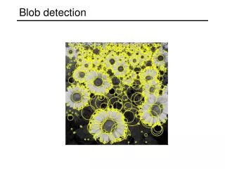
Another kind of feature: blob • “Peak” or “Valley” in intensity
Detecting peaks and valleys • The Laplacian of Gaussian (LoG) (very similar to a Difference of Gaussians (DoG) – i.e. a Gaussian minus a slightly smaller Gaussian)
Scale selection • At what scale does the Laplacian achieve a maximum response for a binary circle of radius r? r image Laplacian
Laplacian of Gaussian minima • “Blob” detector • Find maxima and minima of LoG operator in space and scale * = maximum
Characteristic scale • The scale that produces peak of Laplacian response characteristic scale T. Lindeberg (1998). "Feature detection with automatic scale selection."International Journal of Computer Vision30 (2): pp 77--116.
Find local maxima in position-scale space s5 s4 s3 s2 List of(x, y, s) s K. Grauman, B. Leibe
Matching feature points We know how to detect good points Next question: How to match them? Two interrelated questions: • How do we describe each feature point? • How do we match descriptions? ?
Feature matching • Measure the distance between (or similarity between) every pair of descriptors
Invariance vs. discriminability • Invariance: • Distance between descriptors of corresponding points should be small even if image is transformed • Discriminability: • Descriptor for a point should be highly unique for each point (far away from other points in the image)
Invariance • Most feature descriptors are designed to be invariant to • Translation, 2D rotation, scale • They can usually also handle • Limited 3D rotations (SIFT works up to about 60 degrees) • Limited affine transformations (some are fully affine invariant) • Limited illumination/contrast changes
Simple baseline descriptors Design an invariant feature descriptor • Simplest descriptor: a single 0 • What’s this invariant to? • Is this discriminative? • Next simplest descriptor: a single pixel • What’s this invariant to? • Is this discriminative?
The aperture problem revisited • If we describe the corner by its color alone then it won’t be discriminative • Will it be invariant?
The aperture problem • We can increase the aperture and look at a whole patch • How does this affect discriminability? Invariance?
SSD • Use as descriptor the whole patch • Match descriptors using euclidean distance
NCC - Normalized Cross Correlation • Lighting and color change pixel intensities • Example: increase brightness / contrast • Subtract patch mean: invariance to • Divide by norm of vector: invariance to • similarity =
Basic correspondence • Image patch as descriptor, NCC as similarity • Invariant to? • Photometric transformations? • Translation? • Rotation?
Rotation invariance for feature descriptors • Find dominant orientation of the image patch • This is given by xmax, the eigenvector of M corresponding to max (the larger eigenvalue) • Rotate the patch according to this angle • Figure: line represents xmax, box represents patch we take as feature descriptor Figure by Matthew Brown
Multiscale Oriented PatcheS descriptor Take 40x40 square window around detected feature • Scale to 1/5 size (using prefiltering) • Rotate to horizontal • Sample 8x8 square window centered at feature • Intensity normalize the window by subtracting the mean, dividing by the standard deviation in the window 40 pixels 8 pixels CSE 576: Computer Vision Adapted from slide by Matthew Brown
Scale invariance for feature descriptors • Recall that corner detector searches over scales for maximum response: record scale which gives maximum response • Use a patch of the same scale, then resize it to a fixed size
Multiscale Oriented PatcheS descriptor Take 40x40 square window around detected feature at appropriate scale • Scale to 1/5 size (using prefiltering) • Rotate to horizontal • Sample 8x8 square window centered at feature • Intensity normalize the window by subtracting the mean, dividing by the standard deviation in the window 40 pixels 8 pixels CSE 576: Computer Vision Adapted from slide by Matthew Brown
Feature matching Given a feature in I1, how to find the best match in I2? • Define distance function that compares two descriptors • Test all the features in I2, find the one with min distance