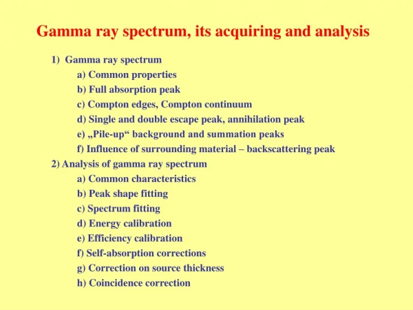
Gamma ray spectrum, its acquiring and analysis

1. Gamma ray spectrum, its acquiring and analysis 1) Gamma ray spectrum a) Common properties b) Full absorption peak c) Compton edges, Compton continuum d) Single and double escape peak, annihilation peak e) „Pile-up“ background and summation peaks f) Influence of surrounding material – backscattering peak 2) Analysis of gamma ray spectrum a) Common characteristics b) Peak shape fitting c) Spectrum fitting d) Energy calibration e) Efficiency calibration f) Self-absorption corrections g) Correction on source thickness h) Coincidence correction

2. Ideal detector – no dead layers, ... • Small detector limit – all secondary photons (from Compton scattering and • annihilation) leave detector Eγ< 2·mec2 Eγ>> 2·mec2 mean free path of secondary photons >> Detector size Ratio of areas of photo peak and Compton background: SF/SC =σF/σC Good resolution (semiconductor) makes possible to see X-ray escape peaks from detector material 2)Large detector limit– all secondary photons are absorbed (very large detector, photons firstly interact at center) Mean free path of secondary photons << detector size All energy is absorbed at the detector

3. Full absorption peak (photo peak) • Gamma quanta interacting by photo effect • Multiple Compton scattering • Pair production and following absorption of annihilation photons Spectrum of 241Am source Spectrum of 60Co source Compton edges One Compton scattering to angle 180O: Two Compton scattering to angle 180O:

4. Spectrum between Compton edges and full absorption peak: • Multiple Compton scattering • Compton scattering at „dead layer“ before detector • Annihilation photons are scattered by Compton scattering • Incomplete charge collection • Escape of characteristic KX - photons Compton continuum Compton background is almost not changing up to Compton edge Many lines → Compton background changes only slowly Spectrum with one line – 137Cs Spectrum with many lines – 152Eu

5. Single and double escape peak Production of electron and positron pair → positron annihilation → two 511 keV photons → one or both escape ESE = E – EA EDE = E – 2·EA kde EA = 511 keV Annihilation peak – 511 keV – broad (electron and positron are not fully in the rest) Characteristic KX rays of detector material Broad peak – set of different transitions on K-shell Important for low energies (photo effect is dominant) X-ray escape lines Important for lower energies and small detector volumes EVR = E – EK EKα(Ge) = 9.885 keV EKβ(Ge) = 10.981 keV

6. „Pile-up effects“ - summation 1) Uncorrelated sums - false coincidences (they are not from the same decay (reaction)) τ– „signal analysis“ τN – „signal creation“ First contribution – stays on energy E Second contribution – move to energy E („pile-up“ spectrum) from sum One line → area of sum peak per time unit: NSP = 2·τ·N2 2) Correlated sums - right coincidences (from the same decay (reaction)) Depends on source decay schema

7. Influence of surrounding materials – backscattering peak Compton scattering in material around sensitive detector volume – marked Peak in the background: Spectrum of gamma ray from 60Co source with backscattering peak and summation peaks 1) Full absorption peaks are placed on relatively slowly varying background 2) Good energy resolution (especially semiconductor) → single peaks occupy small space Resolution of weak lines between intensive ↔ ratio between peak and Compton background

8. Common characteristic Observed spectrum ( S(E’) ) is converted to: E ≤ E´ Digitalization of analog signal: where Wk = Wk1 – Wk0 is channel width – constant is assumed F(E,E´) = G(E,E´) + B(E,E´) where G(E,E´) – absorption of all energies B(E,E´) – incomplete energy conversion Background varies mostly slowly (exception is Compton edges) Background and full absorption peaks are separated in this way

9. We have discrete spectrum of monoenergetic lines: where aj, Ej are intensities and energies of j-th component Measured spectrum: After digitalization: We use analysis of full absorption peaks for determinationof intensities and energies. Approximation by Gauss curve (negligence of natural line width) Eventually different types of step functions or tail to lower energies are added (see rec. literature) Natural width for X-ray is not negligible → its description by Lorentz curve Globally: convolution of Gauss and Lorentz curves Background is approximated by linear function or by higher polynomial, eventually by step

10. Energy calibration Calibration lines (etalons, standards) measured by crystal diffraction spectrometers: Primary standard:198Au 411.8044(11) keV λ = 3010.7788(11) fm Similar also for192Ir, 169Yb a 170Tm – primary calibration sources Eγ = f(k) polynomial, mostly to second order Common measurement of calibration and measured sources Usage of cascade in decay schema Detector efficiency determination Total efficiency εT Efficiency to full absorption peak εF Spectrum purity R = NF/N0 NF - number of registration at full absorption peak N0 – total number of registered photons it is valid:εF = R·εT Certificated calibration sources log-log imaging: log εF = f(log Eγ) Details see recommended literature Example of calibration curve of HPGe detector

11. 4π proportional counter nβ Source NaI(Tl) nc Photomultiplier nγ Absoluteactivity determination Assumptions – every decay one beta and one gamma conversion coefficient is negligible one detector cleanly for electrons (gas) second detects only gamma photons Number of detected electrons: nβ = Aεβ Number of detected gamma photons:nγ = Aεγ Number of coincidences of electron and photon detections: nc = A·εβεγ Afterwards absolute activity of source is:

12. Correction on uncertainty of source position and thickness: Equation for solid angle: and then: Details see recommended literature Selfabsorption correction: Gamma intensity decreasing done by absorption (μ – linear absorption coefficient): Source with homogenous thickness Dis assumed: correction coefficient is: Coincidence correction: Details see recommended literature and exercise