Download
1 / 19
190 likes | 285 Vues
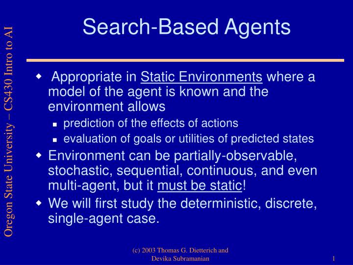
Search-Based Agents. Appropriate in Static Environments where a model of the agent is known and the environment allows prediction of the effects of actions evaluation of goals or utilities of predicted states

E N D
Search-Based Agents • Appropriate in Static Environments where a model of the agent is known and the environment allows • prediction of the effects of actions • evaluation of goals or utilities of predicted states • Environment can be partially-observable, stochastic, sequential, continuous, and even multi-agent, but it must be static! • We will first study the deterministic, discrete, single-agent case. (c) 2003 Thomas G. Dietterich and Devika Subramanian
Oradea 71 Neamt 87 Zerind 151 75 Iasi Arad 140 92 Sibiu Fagaras 99 118 Vasini 80 Rimnicu Vilcea Timisoara 142 211 111 Pitesti Lugoj 97 70 98 Hirsova 85 146 Mehadia 101 Urzicenl 86 75 138 Bucharest Dobreta 120 90 Eforie Craiova Giurgia Computing Driving Directions You are here You want to be here (c) 2003 Thomas G. Dietterich and Devika Subramanian
Search Algorithms • Breadth-First • Depth-First • Uniform Cost • A* • Dijkstra’s Algorithm (c) 2003 Thomas G. Dietterich and Devika Subramanian
Oradea (146) 71 Zerind (75) 151 75 Arad (0) 140 Sibiu (140) Fagaras (239) 99 118 80 Rimnicu Vilcea (220) Timisoara (118) Pitesti (317) 211 111 Lugoj (229) 97 70 Mehadia (299) 146 101 75 138 Bucharest (450) Dobreta (486) 120 Craiova (366) Breadth-First Detect duplicate path (291) Detect duplicate path (197) Detect new shorter path (418) Detect duplicate path (504) Detect new shorter path (374) Detect duplicate path (455) Detect duplicate path (494) (c) 2003 Thomas G. Dietterich and Devika Subramanian
Oradea (146) 71 Zerind (75) 151 75 Arad (0) 140 Sibiu (140) Fagaras (239) 99 118 80 Rimnicu Vilcea (220) Timisoara (118) Zerind (75) Sibiu (140) Timisoara (118) Pitesti (317) 211 111 Lugoj (229) 97 Arad (150) Oradea (146) Arad (280) Fagaras (239) Oradea (291) Arad (236) Lugoj (229) Rimnicu Vilcea (220) 70 Mehadia (299) 146 101 Sibiu (197) Sibiu (338) Bucharest (450) Timisoara (340) Mehadia (299) Zerind (217) Sibiu (300) Pitesti (317) Craiova (366) 75 138 Bucharest (450) Dobreta (486) 120 Lugoj (369) Dobreta (374) Craiova (366) Rimnicu Vilcea (482) Rimnicu Vilcea (317) Bucharest (418) Craiova (455) Dobreta (486) Pitesti (504) Medhadia (449) Craiova (494) Breadth-First Arad (0)
Formal Statement of Search Problems • State Space: set of possible “mental” states • cities in Romania • Initial State: state from which search begins • Arad • Operators: simulated actions that take the agent from one mental state to another • traverse highway between two cities • Goal Test: • Is current state Bucharest? (c) 2003 Thomas G. Dietterich and Devika Subramanian
General Search Algorithm • Strategy: first-in first-out queue (expand oldest leaf first) (c) 2003 Thomas G. Dietterich and Devika Subramanian
Leaf Selection Strategies • Breadth-First Search: oldest leaf (FIFO) • Depth-First Search: youngest leaf (LIFO) • Uniform Cost Search: cheapest leaf (Priority Queue) • A* search: leaf with estimated shortest total path length g(x) + h(x) = f(x) • where g(x) is length so far • and h(x) is estimate of remaining length • (Priority Queue) (c) 2003 Thomas G. Dietterich and Devika Subramanian
A* Search • Let h(x) be a “heuristic function” that gives an underestimate of the true distance between x and the goal state • Example: Euclidean distance • Let g(x) be the distance from the start to x, then g(x) + h(x) is an lower bound on the length of the optimal path (c) 2003 Thomas G. Dietterich and Devika Subramanian
Euclidean Distance Table (c) 2003 Thomas G. Dietterich and Devika Subramanian
Fagaras (239+176=415) Oradea (291+380=671) Rimnicu Vilcea (220+193=413) Pitesti (317+100=417) Zerind (75+374=449) Sibiu (140+253=393) Timisoara (118+329=447) Craiova (455+160=615) Bucharest (450+0=450) Craiova (366+160=526) Bucharest (418+0=418) A* Search Arad (0+366=366) All remaining leaves have f(x)¸ 418, so we know they cannot have shorter paths to Bucharest (c) 2003 Thomas G. Dietterich and Devika Subramanian
Dijkstra’s Algorithm • Works backwards from the goal • Each node keeps track of the shortest known path (and its length) to the goal • Equivalent to uniform cost search starting at the goal • No early stopping: finds shortest path from all nodes to the goal (c) 2003 Thomas G. Dietterich and Devika Subramanian
Local Search Algorithms • Keep a single current state x • Repeat • Apply one or more operators to x • Evaluate the resulting states according to an Objective FunctionJ(x) • Choose one of them to replace x (or decide not to replace x at all) • Until time limit or stopping criterion (c) 2003 Thomas G. Dietterich and Devika Subramanian
Hill Climbing • Simple hill climbing: apply a randomly-chosen operator to the current state • If resulting state is better, replace current state • Steepest-Ascent Hill Climbing: • Apply all operators to current state, keep state with the best value • Stop when no successors state is better than current state (c) 2003 Thomas G. Dietterich and Devika Subramanian
Gradient Ascent • In continuous state spaces, x = (x1, x2, …, xn) is a vector of real values • Continuous operator: x := x+ x for any arbitrary vector x (infinitely many operators!) • Suppose J(x) is differentiable. Then we can compute the direction of steepest increase of J by the first derivative with respect to x, the gradient: (c) 2003 Thomas G. Dietterich and Devika Subramanian
Gradient Descent Search • Repeat • Compute Gradient rJ • Update x := x + rJ • Until rJ ¼ 0 • is the “step size”, and it must be chosen carefully • Methods such as conjugate gradient and Newton’s method choose automatically (c) 2003 Thomas G. Dietterich and Devika Subramanian
Visualizing Gradient Ascent If is too large, search may overshoot and miss the maximum or oscillate forever (c) 2003 Thomas G. Dietterich and Devika Subramanian
Problems with Hill Climbing • Local optima • Flat regions • Random restarts can give good results (c) 2003 Thomas G. Dietterich and Devika Subramanian
Simulated Annealing • T = 100 (or some large value) • Repeat • Apply randomly-chosen operator to x to obtain x′. • Let E = J(x′) – J(x) • If E > 0, /* J(x′) is better */ switch to x′ • Else /* J(x′) is worse */ switch to x′ with probability • exp [E/T] /* large negative steps are less likely */ • T := 0.99 * T */ “cool” T */ • Slowly decrease T (“anneal”) to zero • Stop when no changes have been accepted for many moves • Idea: Accept “down hill” steps with some probability to help escape from local minima. As T ! 0 this probability goes to zero. (c) 2003 Thomas G. Dietterich and Devika Subramanian