Download
1 / 5
50 likes | 138 Vues
> xyplot(cat~time|id,dd,groups=ses,lty=1:3,type="l") > dd<-read.csv("c:\minna\longitudinal\comp.csv") > head(dd) id ses cat pre post time 1 430 1 6 21 0 1 2 430 1 6 21 0 2 3 430 1 6 21 0 3 4 430 1 6 21 0 4 5 430 1 6 21 0 5

E N D
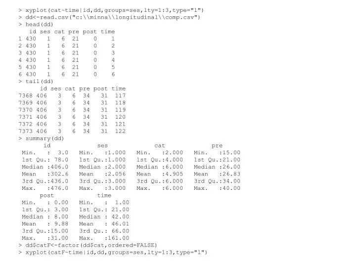
> xyplot(cat~time|id,dd,groups=ses,lty=1:3,type="l") > dd<-read.csv("c:\\minna\\longitudinal\\comp.csv") > head(dd) id ses cat pre post time 1 430 1 6 21 0 1 2 430 1 6 21 0 2 3 430 1 6 21 0 3 4 430 1 6 21 0 4 5 430 1 6 21 0 5 6 430 1 6 21 0 6 > tail(dd) id ses cat pre post time 7368 406 3 6 34 31 117 7369 406 3 6 34 31 118 7370 406 3 6 34 31 119 7371 406 3 6 34 31 120 7372 406 3 6 34 31 121 7373 406 3 6 34 31 122 > summary(dd) id ses cat pre Min. : 3.0 Min. :1.000 Min. :2.000 Min. :15.00 1st Qu.: 78.0 1st Qu.:1.000 1st Qu.:4.000 1st Qu.:21.00 Median :406.0 Median :2.000 Median :6.000 Median :26.00 Mean :302.6 Mean :2.056 Mean :4.905 Mean :26.83 3rd Qu.:436.0 3rd Qu.:3.000 3rd Qu.:6.000 3rd Qu.:34.00 Max. :476.0 Max. :3.000 Max. :6.000 Max. :40.00 post time Min. : 0.00 Min. : 1.00 1st Qu.: 3.00 1st Qu.: 21.00 Median : 8.00 Median : 42.00 Mean : 9.88 Mean : 46.01 3rd Qu.:15.00 3rd Qu.: 66.00 Max. :31.00 Max. :161.00 > dd$catF<-factor(dd$cat,ordered=FALSE) > xyplot(catF~time|id,dd,groups=ses,lty=1:3,type="l")
Problem:time | patient + sessiondiffers, how to deal with this? > mod <- lmer( catF ~ time*ses+pre+post+(time|id),dd) Error in checkSlotAssignment(object, name, value) : assignment of an object of class "factor" is not valid for slot 'y' in an object of class "lmer"; is(value, "numeric") is not TRUE > mod <- lmer( cat ~ time*ses+pre+post+(time|id),dd) > summary(mod) Linear mixed-effects model fit by REML Formula: cat ~ time * ses + pre + post + (time | id) Data: dd AIC BIC logLik MLdeviance REMLdeviance 26286 26349 -13134 26223 26268 Random effects: Groups Name Variance Std.Dev. Corr id (Intercept) 0.46120448 0.679120 time 0.00014212 0.011921 -0.692 Residual 2.00449172 1.415801 number of obs: 7373, groups: id, 30
Fixed effects: Estimate Std. Error t value (Intercept) 4.7387891 0.4203240 11.274 time 0.0054949 0.0027672 1.986 ses 0.0309587 0.0379076 0.817 pre -0.0054968 0.0139072 -0.395 post 0.0140585 0.0109736 1.281 time:ses -0.0016274 0.0007328 -2.221 Correlation of Fixed Effects: (Intr) time ses pre post time -0.257 ses -0.184 0.459 pre -0.896 -0.009 0.000 post -0.316 0.006 -0.001 0.057 time:ses 0.151 -0.562 -0.835 0.009 -0.004 > anova(mod) Analysis of Variance Table Df Sum Sq Mean Sq time 1 1.4400 1.4400 ses 1 6.9715 6.9715 pre 1 0.4105 0.4105 post 1 3.2776 3.2776
Questions: • Length | patient+session are different, how to deal with it? Missing data? • How to analyze the categorical response? • How to make a better plot? • Can we look at the proportion of each categories? • Can we look at the sequence of the change of the categories? – can we model this as Markov chain? • Compare each session for each patients