Download
1 / 37
380 likes | 993 Vues
Parameter estimation for HMMs, Baum-Welch algorithm, Model topology, Numerical stability . Chapter 3.3-3.7. Overview . Parameter estimation for HMMs Baum-Welch algorithm HMM model structure More complex Markov chains Numerical stability of HMM algorithms. Specifying a HMM model.

E N D
Parameter estimation for HMMs, Baum-Welch algorithm, Model topology, Numerical stability Chapter 3.3-3.7 Elze de Groot
Overview • Parameter estimation for HMMs • Baum-Welch algorithm • HMM model structure • More complex Markov chains • Numerical stability of HMM algorithms Elze de Groot
Specifying a HMM model • Most difficult problem using HMMs is specifying the model • Design of the structure • Assignment of parameter values Elze de Groot
Specifying a HMM model • Most difficult problem using HMMs is specifying the model • Design of the structure • Assignment of parameter values Elze de Groot
Parameter estimation for HMMs • Estimate transition and emission probabilities akl and ek(b) • Two ways of learning: • Estimation when state sequence is known • Estimation when paths are unknown • Assume that we have a set of example sequences (training sequences x1, …xn) Elze de Groot
Parameter estimation for HMMs • Assume that x1…xnindependent. • joint probability • Log space Since log ab = log a + logb Elze de Groot
Estimation when state sequence is known • Easier than estimation when paths unknown • Akl= number of transitions k to l in trainingdata + rkl • Ek(b) = number of emissions of b from k in training data + rk(b) Elze de Groot
Estimation when paths are unknown • More complex than when paths are known • We can’t use maximum likelihood estimators • Instead, an iterative algorithm is used • Baum-Welch Elze de Groot
The Baum-Welch algorithm • We don’t know real values of Akl and Ek(b) • Estimate Akl and Ek(b) • Update akl and ek(b) • Repeat with new model parameters akl and ek(b) Elze de Groot
Forward value Backward value Baum-Welch algorithm Elze de Groot
Baum-Welch algorithm • Now that we have estimated Akl and Ek(b), use maximum likelihood estimators to compute akl and ek(b) • We use these values to estimate Akl and Ek(b) in the next iteration • Continue doing this iteration until change is very small or max number of iterations is exceeded Elze de Groot
Baum-Welch algorithm Elze de Groot
Example • Estimated model with 300 rolls and 30.000 rolls Elze de Groot
Drawbacks • ML estimators • Vulnerable to overfitting if not enough data • Estimations can be undefined if never used in training set (so use of pseudocounts) • Baum-Welch • Many local maximums instead of global maximum can be found, depending on starting values of parameters • This problem will be worse for large HMMs Elze de Groot
Viterbi Training • Most probable path derived using viterbi algorithm • Continue until none of paths change • Finds value of θ that maximises contribution to likelihood • Performs less well than baum welch Elze de Groot
Modelling of labelled sequences • Only -- and ++ are calculated • Better than using ML estimators, when many different classes are present Elze de Groot
Specifying a HMM model • Most difficult problem using HMMs is specifying the model • Design of the structure • Assignment of parameter values Elze de Groot
Design of the structure • Design: how to connect states by transitions • A good HMM is based on the knowledge about the problem under investigation • Local maxima are biggest disadvantage in models that are fully connected • After deleting a transition from model Baum-Welch will still work: set transition probability to zero Elze de Groot
p 1-p Example 1 • Geometric distribution Elze de Groot
Example 2 • Model distribution of length between 2 and 10 Elze de Groot
Example 3 • Negative binomial distribution • p=0.99 • n≤5 Elze de Groot
B Silent states • States that do not emit symbols • Also in other places in HMM Elze de Groot
Silent states Example Elze de Groot
Silent states • Advantage: • Less estimations of transition probabilities needed • Drawback: • Limits the possibilities of defining a model Elze de Groot
Silent states • Change in forward algorithm • For ‘real’ states the same • For silent states set • Starting from lowest numbered silent state l add for all silent states k<l Elze de Groot
More complex Markov chains • So far, we assumed that probability of a symbol in a sequence depends only on the probability of the previous symbol • More complex • High order Markov chains • Inhomogeneous Markov chains Elze de Groot
P(AB|B) = P(A|B) High order Markov chains • An nth order Markov process • Probability of a symbol in a sequence depends on the probability of the previous n symbols • An nth order Markov chain over some alphabet A is equivalent to a first order Markov chain over the alphabet Anof n-tuples, because: Elze de Groot
Example • A second order Markov chain with two different symbols {A,B} • This can be translated into a first order Markov chain of 2-tuples {AA, AB, BA, BB} Sometimes the framework of high order model is convenient Elze de Groot
Finding prokaryotic genes • Gene candidates in DNA: -sequence of triplets of nucleotides: startcodon nr. of non-stopcodons stopcodon -open reading frame (ORF) • An ORF can be either a gene or a non-coding ORF (NORF) Elze de Groot
Finding prokaryotic genes • Experiment: • DNA from bacterium E.coli • Dataset contains 1100 genes (900 used for training, 200 for testing) • Two models: • Normal model with first order Markov chains • Also first order Markov chains, but codons instead of nucleotides are used as symbol Elze de Groot
Finding prokaryotic genes • Outcomes: Elze de Groot
CAT GCA P(C)aCA aAT aTG aGC aCA P(C)a2CA a3AT a1TG a2GC a3CA Inhomogeneous Markov chains • Using the position information in the codon • Three models for position 1, 2 and 3 1 2 3 1 2 3 Homogeneous Inhomogeneous Elze de Groot
Numerical Stability of HMM algorithms • Multiplying many probabilities can cause numerical problems: • Underflow errors • Wrong numbers are calculated • Solutions: • Log transformation • Scaling of probabilities Elze de Groot
The log transformation • Compute log probabilities • Log 10-100000 = -100000 • Underflow problem is essentially solved • Sum operation is often faster than product operation • In the Viterbi algorithm: Elze de Groot
Scaling of probabilities • Scale f and b variables • Forward variable: • For each i a scaling variable si is defined • New f variables are defined: • New forward recursion: Elze de Groot
Scaling of probabilities • Backward variable • Scaling has to be with same numbers as forward variable • New backward recursion: • This normally works well, however underflow errors can still occur in models with many silent states (chapter 5) Elze de Groot
Summary • Hidden Markov Models • Parameter estimation • State sequence known • State sequence unknown • Model structure • Silent states • More complex Markov chains • Numerical stability Elze de Groot