Download
1 / 24
240 likes | 346 Vues
An Examination Of Interesting Properties Regarding A Physics Ensemble. 2012 WRF Users’ Workshop Nick P. Bassill June 28 th , 2012. Introduction. During the 2009 North Atlantic hurricane season, a real-time ensemble was created locally once per day

E N D
An Examination Of Interesting Properties Regarding A Physics Ensemble 2012 WRF Users’ Workshop Nick P. Bassill June 28th, 2012
Introduction • During the 2009 North Atlantic hurricane season, a real-time ensemble was created locally once per day • Using simple linear regression techniques, I will present a few (potentially) interesting results comparing a low resolution WRF-ARW physics ensemble with the operation GFS ensemble
Data Generation Overview Dynamical Core is WRF-ARW 3.0 Two Days Between Each Initialization (From GFS 00Z Forecast) 76 Cases From Early June Through October Initialization Time Spread Of 120 Hour Forecasts
Outer Domain: 90 km Grid Spacing Inner Domain: 30 km Grid Spacing
Physics Ensemble vs. GFS Ensemble • The results shown were calculated as follows:- Tune 120 hour forecasts to 0 hour GFS analyses for both the physics ensemble* and GFS ensemble comprised of an equal number of members - After this is done, it’s easy to calculate the average error per case for both ensembles - The average error will be shown, along with the difference between the two normalized to the standard deviation of the variable in question * Using outer 90 km grid
2 Meter Temperature (°C) • (Left): Yellow and red colors mean the parameterization ensemble outperformed the GFS ensemble, blue colors mean the opposite
500 hPa Geopotential Height (m) • (Right): Yellow and red colors mean the parameterization ensemble outperformed the GFS ensemble, blue colors mean the opposite
10 Meter Wind Speed (m/s) • (Left): Yellow and red colors mean the parameterization ensemble outperformed the GFS ensemble, blue colors mean the opposite
Observations • On average, the GFS ensemble “wins” by ~0.01 standard deviations for any given variable • Generally speaking, the parameterization ensemble performs better in the tropics, while the GFS ensemble performs better in the sub/extratropics Let’s examine the 2 m temperature more closely …
2 Meter Temperature Composites • The fill is the mean 2 m temperature at hour 120 for the parameterization ensemble members • The contour is the 95% significance threshold
2 Meter Temperature Composites • The fill is the mean 2 m temperature anomaly at hour 120 for the parameterization ensemble members • The contour is the 95% significance threshold as seen previously
2 Meter Temperature Composites • The fill is the mean 2 m temperature anomaly at hour 120 for the parameterization ensemble members • The contour is the 95% significance threshold as seen previously
2 Meter Temperature Composites • The fill is the mean 2 m temperature at hour 120 for the GFS ensemble members • Note – no significance contour is shown
2 Meter Temperature Composites • The fill is the mean 2 m temperature anomaly at hour 120 for the GFS ensemble members • Note how indistinguishable one member is from another • Unlike the physics ensemble, member differences aren’t correlated from run to run
Parameterization Ensemble Member Errors Black = YSU PBL Members At ~44 N, -108 W Green = MYJ PBL Members
Conclusions • Different parameterization combinations do have certain (statistically significant) biases • Pure parameterization ensembles theoretically are better than pure initial condition ensembles, since member differences are correlated from run to run • Using this information, a simple (read: dumb) parameterization ensemble can perform equivalently to a “superior” ensemble • This is done by viewing parameterization biases as a benefit, not a problem
Future Work • Currently, the parameterization ensemble vs. GFS ensemble results are being redone with the use of Global WRF • More advanced statistical techniques could be used to improve on these results - Unequal weighting - Using more predictors - Identifying regimes
WSM3 Microphysics Parameterization Ferrier Microphysics Parameterization Kain-Fritsch Cumulus Parameterization MYJ Boundary Layer Parameterization Betts-Miller-Janjic Cumulus Parameterization YSU Boundary Layer Parameterization Grell-3 Cumulus Parameterization
Idea: Predicting Predictions • Generically speaking, all of these models are pretty similar • For each forecast day, I ran an additional model with completely different parameterizations, which were purposely chosen to be “bad” (at least in combination) • Afterward, I used the original ten models to predict the new one (i.e. a prediction of a prediction) using multivariate linear regression