Download
1 / 8
80 likes | 282 Vues
LP Examples Solid Waste Management. A SOLID WASTE PROBLEM. A city generates 200 tons/day of solid wastes and must dispose it to three landfills . The data about the cost is given in the table. For environmental reason all the three landfills has to be utilized.

E N D
A SOLID WASTE PROBLEM A city generates 200 tons/day of solid wastes and must dispose it to three landfills. The data about the cost is given in the table. For environmental reason all the three landfills has to be utilized. Develop the needed equations (objective function and constraints) for Linear programming model to find the optimal distribution of the waste to the three landfills.
MODEL FORMULATION • MIN 7 X1 + 8 X2 + 6 X3 • SUBJECT TO X1 + X2 + X3 = 200 X1 <= 120 X2 <= 100 X3 <= 50 X1 >= 0 X2 >= 0 X3 >= 0 • END
SOLID WASTE SOLUTION using LINDO Objective function Value = $1380 X1 = 120; X2 = 30; X3 = 50
SOIL STABILITY PROBLEM • In order to assure adequate stability under load repetition, a soil mixture for base and sub-base courses in the construction of a certain highway must have a liquid limit, 21=<LL<=28, and a Plasticity Index, 4=<PI<=6. • Two materials, A and B, are available as follows: • Properties A B • LL 35 20 • PI 8 3.5 • Cost ($/cu. m ) $.35 $.65 • Assume that the LL and the PI are linear functions of the combinations of the two materials A and B and determine the optimal proportion of base and sub-base.
MODEL FORMULATION MIN 0.35 XA + 0.65 XB SUBJECT TO L.L. 35 XA + 20 XB >= 21 L.L. 35 XA + 20 XB <= 28 P.I. 8 XA + 3.5 XB >= 4 P.I. 8 XA + 3.5 XB <= 6 Proportionality XA + XB = 1 END
Case 2: LINDO OUTPUT SOLUTION: LP OPTIMUM FOUND AT STEP 4 OBJECTIVE FUNCTION VALUE 1) .4900000 VARIABLE VALUE REDUCED COST XA .533333 .000000 XB .466667 .000000 ROW SLACK OR SURPLUS DUAL PRICES 2) 7.000000 .000000 3) .000000 .020000 4) 1.900000 .000000 5) .100000 .000000 6) .000000 -1.050000 NO. ITERATIONS= 4 RANGE(SENSITIVITY) ANALYSIS: Y ? :RANGES IN WHICH THE BASIS IS UNCHANGED OBJ COEFFICIENT RANGES VARIABLE CURRENT ALLOWABLE ALOWABLE COEF INCREASE DECREASE XA .350000 .300000 INFINITY XB .650000 INFINITY .300000 RIGHTHAND SIDE RANGES ROW CURRENT ALLOWABLE ALOWABLE RHS INCREASE DECREASE 2 21.000000 7.000000 INFINITY 3 28.000000 .333333 6.333333 4 4.000000 1.900000 INFINITY 5 6.000000 INFINITY .100000 6 1.000000 .400000 .040000