Download
1 / 23
230 likes | 417 Vues
Cloud Top Properties. Bryan A. Baum NASA Langley Research Center Paul Menzel NOAA Richard Frey, Hong Zhang CIMSS University of Wisconsin-Madison. MODIS Science Team Meeting July 13-15 2004. CO 2 Slicing: Cloud Pressure and Effective Cloud Amount. CO 2 slicing method

E N D
Cloud Top Properties Bryan A. Baum NASA Langley Research Center Paul Menzel NOAA Richard Frey, Hong Zhang CIMSS University of Wisconsin-Madison MODIS Science Team Meeting July 13-15 2004
CO2 Slicing: Cloud Pressure and Effective Cloud Amount • CO2 slicing method • long-term operational use • ratio of cloud signals at two near-by wavelengths • retrieve Pc and A (product of cloud emittance and cloud fraction A) • The technique is most accurate for mid- and high-level clouds • Pressure related to temperature via the GDAS gridded meteorological product • MODIS is the first sensor to have CO2 slicing bands at high spatial resolution (1 km)
14 Jan 2003: thin high cloudMODIS CTP too low at thin cloud edges Dr. Catherine Naud, visiting CIMSS during the summer of 2003, intercompared MODIS, MISR and MERIS. One of her findings was that in Collection 4, cloud top pressures tended to decrease near cirrus edges, (in other words, cirrus cloud heights “curled up” at the boundaries as the clouds thinned out).
Improvements to the Algorithm for Collect 5 As a result of Catherine’s work, resolution of the issue led to numerous changes. Apply new forward model coefficients (LBLRTM version 7.4) • - employed new 101 pressure-level forward model (old model had 42 levels) • - changed transmittance profile characteristics significantly • - end result is that pressures are much more consistent as clouds thin out Read in all levels of GDAS temperature and moisture profiles - needed to rework use of GDAS for 101-level model Reduce total number of forward model calculations for efficiency - required for operational processing; also necessary in case we move to 1-km processing SSTs, GDAS land surface temperatures and pressures are bilinearly interpolated - but we still have issues over land
Improvements to the Algorithm for Collect 5 Another issue: low-level cloud pressure/temperature/height If CO2 slicing is not performed, and a cloud is thought to be present, then the 11-m band is used to infer cloud top temperature/pressure assuming the cloud is opaque Collection 4 (not yet operational forTerra, but fixed for Aqua): - compare measured 11-m brightness temperature to the GDAS temperature profile Collection 5: - account for water vapor absorption in 11-m band using the 101-level forward model - compare measured to calculated 11-m radiance - result is more accurate low-cloud assessments
Simulations of Ice and Water Phase Clouds 8.5 - 11 m BT Differences • High Ice clouds • BTD[8.5-11] > 0 over a large range of optical thicknesses • Tcld = 228 K = • Midlevel clouds • BTD[8.5-11] values are similar (i.e., negative) for both water and ice clouds • Tcld = 253 K • Low-level, warm clouds • BTD[8.5-11] values always negative • Tcld = 273 K = Ice: Cirrus model derived from FIRE-I in-situ data * Water: re=10 mm Angles: o = 45o, = 20o, and = 40o Profile: midlatitude summer *Nasiri et al, 2001
MODIS Cloud Thermodynamic Phase Percentage Ice and Water Cloud 05 Nov. 2000 -Daytime Only frequency of occurrence in percent (%)
MODIS Cloud Thermodynamic Phase Percentage Ice and Water Cloud 05 Nov. 2000 - Nighttime Only frequency of occurrence in percent (%)
MODIS Frequency of Co-occurrence Water Phase with 253 K < Tcld < 268 K 05 Nov. 2000 - Daytime Only frequency of occurrence in percent (%)
MODIS Frequency of Co-occurrence Water Phase with 253 K < Tcld < 268 K 05 Nov. 2000 - Nighttime Only frequency of occurrence in percent (%)
MODIS Daytime Cloud Overlap Technique • Assumption: At most 2 cloud layers in data array • For a 200x200 pixel (1km resolution) array of MODIS data: • Identify clear pixels from MODIS cloud mask • Identify unambiguous ice pixels and water pixels from the 8.5- and 11-m bispectral cloud phase technique • Classify unambiguous ice/water pixels as belonging to the higher/lower cloud layer • Classify remaining pixels as overlapped • Stagger the pixel array over the image so that each pixel is analyzed multiple times (away from the granule borders)
MAS data from single-layered cirrus and water phase clouds • 1.6 µm reflectance varies as a function of optical thickness more for water clouds than ice clouds • 11 µm BT varies as a function of optical thickness more for ice clouds than for water clouds RT simulation of a water cloud RT simulation of a cirrostratus cloud From Baum and Spinhirne (2000), Figure 2a
MAS data from cirrus overlying water phase cloud • MAS data from overlap region falls between single layer water and cirrus cloud data in R[1.63 µm] and BT[11 µm] space RT simulation of a water cloud RT simulation of a cirrostratus cloud From Baum and Spinhirne (2000), Figure 2b
0.8 0.6 0.4 0.2 0 200 by 200 pixels of MODIS Data from 15 Oct. 2000 at 1725Z Water Cloud (from MODIS Phase) Ice Cloud (from MODIS Phase) Clear (from MODIS Cloud Mask) 1.6 m Reflectance Other (to be determined) 210 230 250 270 290 11 m BT (K)
Recent Research Greg McGarragh has been producing the following products using MODIS Direct Broadcast at 1 km resolution for the past year a. Daytime multilayered cloud identification b. Cloud phase c. Cloud top pressure and effective cloud amount Note: The products are greatly improved by incorporating the CIMSS destriping software on all IR bands. The multilayered cloud and IR cloud phase are being incorporated in the DB operational software, and will eventually go into DAAC operational code
MODIS Terra Over Western U.S. on 6 July 2004 - 1842 UTC Effective Cloud Amount Pressure (hPa) RGB: Bands 1, 7, 31(flipped)
MODIS Terra Over Western U.S. on 6 July 2004 - 1842 UTC Pressure (hPa)
MODIS Terra Over Western U.S. on 6 July 2004 - 1842 UTC Pressure (hPa)
MODIS Terra Over Western U.S. on 6 July 2004 - 1842 UTC Pressure (hPa)
April 1-8, 2003 8-day composite Aqua Frequency of CTP < 440 hPa & A < 0.5 Frequency of multilayered cloud detection frequency of occurrence in percent (%)
MODIS Aqua, April 1-8, 2003 Multilayered clouds: breakdown by IR-derived phase Ice phase Water phase Mixed phase Uncertain phase
ISCCP (top), HIRS (mid), & MODIS (bot) for July (left) & Dec (right) 2002
Summary of Improvements to the CTP for Collect 5 • Apply new forward model coefficients (LBLRTM version 7.4) • Read in all levels of GDAS temperature and moisture profiles • Reduce total number of forward model calculations for efficiency • SSTs, GDAS land surface temperatures and pressures are bi-linearly interpolated • Apply simple land vs. water surface emissivity correction • Account for water vapor absorption in window band calculations • Reduced Aqua noise thresholds (allowable clear vs. cloudy radiance differences) • Employ UW-Madison de-striping algorithm for L1b input radiances