Download
1 / 62
620 likes | 717 Vues
Cryptosystems from unique-SVP lattices Ajtai-Dwork’97/07, Regev’03. Many slides borrowed from Oded Regev, denoted by. Shai Halevi, MIT, August 2009. . 1. f(n). . f(n)-unique-SVP. Promise: the shortest vector u is shorter by a factor of f(n)

E N D
Cryptosystems from unique-SVP latticesAjtai-Dwork’97/07, Regev’03 Many slides borrowed from Oded Regev, denoted by Shai Halevi, MIT, August 2009
1 f(n) f(n)-unique-SVP • Promise: the shortest vector u is shorter by a factor of f(n) • Algorithm for 2n-unique SVP [LLL82,Schnorr87] • Believed to be hard for any polynomial nc nc 2n 1 believed hard easy
Worst-case Search u-SVP Worst-case Decision u-SVP Regev03: “Hensel lifting” AD97: Geometric Basic Intuition “Worst-case Distinguisher” Wavy-vs-Uniform Leftover hash lemma AD97 PKE bit-by-bit n-dimensional Amortizing by adding dimensions Projecting to a line Regev03 PKE bit-by-bit 1-dimensional AD07 PKE O(n)-bits n-dimensional Ajtai-Dwork & Regev’03 PKEs Nearly-trivial worst-case/average-case reductions
n-dimensional distributions • Distinguish between the distributions: ? Uniform Wavy (In a random direction)
Dual Lattice • Given a lattice L, the dual lattice is L* = { x | for all yL, <x,y>Z } 1/5 L L* 5 0 0
L* - the dual of L L* L n 0 Case 1 1/n 0 n n Case 2 0
Reduction • Input: a basis B* for L* • Produce a distribution that is: • Wavy if L has unique shortest vector (|u|1/n) • Uniform (on P(B*)) if l1(L) > n • Choose a point from a Gaussian of radius n, and reduce mod P(B*) • Conceptually, a “random L* point” with a Gaussian(n) perturbation
Creating the Distribution L* L*+ perturb 0 Case 1 n Case 2
Analyzing the Distribution • Theorem: (using [Banaszczyk’93]) The distribution obtained above depends only on the points in L of distance n from the origin (up to an exponentially small error) • Therefore, Case 1: Determined by multiples of u wavy on hyperplanes orthogonal to u Case 2: Determined by the origin uniform
Proof of Theorem • For a set A in Rn,define: • Poisson Summation Formula implies: • Banaszczyk’s theorem: For any lattice L,
Proof of Theorem (cont.) • In Case 2, the distribution obtained is very close to uniform: • Because:
Worst-case Search u-SVP Worst-case Decision u-SVP Regev03: “Hensel lifting” AD97: Geometric Basic Intuition “Worst-case Distinguisher” Wavy-vs-Uniform Ajtai-Dwork & Regev’03 PKEs next
DistinguishSearch, AD97 • Reminder: L* lives in hyperplanes • We want to identify u • Using an oracle that distinguishes wavy distributions from uniform in P(B*) u H1 H0 H-1
The plan • Use the oracle to distinguish points close to H0 from points close to H1 • Then grow very long vectors that are rather close to H0 • This gives a very good approximationfor u, then we use it to find u exactly
Distinguishing H0 from H1 Input: basis B* for L*, ~length of u, point x • And access to wavy/uniform distinguisher Decision: Is x 1/poly(n) close to H0 or to H1? • Choose y from a wavy distribution near L* • y = Gaussian(s)* with s < 1/2|u| • Pick aR[0,1], set z = ax + y mod P(B*) • Ask oracle if z is drawn from wavy or uniform distribution * Gaussian(s): variance s2 in each coordinate
Distinguishing H0 from H1 (cont.) Case 1: x close to H0 • ax also close to H0 • ax + y mod P(B*) close to L*, wavy x H0
Distinguishing H0 from H1 (cont.) Case 2: x close to H1 • ax “in the middle” between H0 and H1 • Nearly uniform component in the u direction • ax + y mod P(B*) nearly uniform in P(B*) x H1 H0
Distinguishing H0 from H1 (cont.) • Repeat poly(n) times, take majority • Boost the advantage to near-certainty • Below we assume a “perfect distinguisher” • Close to H0 always says NO • Close to H1 always says YES • Otherwise, there are no guarantees • Except halting in polynomial time
Growing Large Vectors • Start from some x0 between H-1 and H+1 • e.g. a random vector of length 1/|u| • In each step, choose xi s.t. • |xi| ~ 2|xi-1| • xi is somewhere between H-1 and H+1 • Keep going for poly(n) steps • Result is x* between H1 with |x*|=N/|u| • Very large N, e.g., N=2n we’ll see how in a minute 2
From xi-1 to xi Try poly(n) many candidates: • Candidate w = 2xi-1 + Gaussian(1/|u|) • For j = 1,…, m=poly(n) • wj = j/m · w • Check if wj is near H0 or near H1 • If none of the wj’s is near H1 then accept w and set xi = w • Else try another candidate w=wm w2 w1
From xi-1 to xi: Analysis • xi-1 between H1 w is between Hn • Except with exponentially small probability • w is NOT between H1 some wj near H1 • So w will be rejected • So if we make progress, we know that we are on the right track
From xi-1 to xi: Analysis (cont.) • With probability 1/poly(n), w is close to H0 • The component in the u direction is Gaussianwith mean < 2/|u| and variance 1/|u|2 noise 2xi-1 H1 H0
From xi-1 to xi: Analysis (cont.) • With probability 1/poly, w is close to H0 • The component in the u direction is Gaussianwith mean < 2/|u| and standard deviation 1/|u| • w is close to H0, all wj’s are close to H0 • So w will be accepted • After polynomially many candidates, we will make progress whp
Finding u • Find n-1 x*’s • x*t+1 is chosen orthogonal to x*1,…,x*t • By choosing the Gaussians in that subspace • Compute u’ {x*1,…,x*n-1}, with |u’|=1 • u’ is exponentially close to u/|u| • u/|u| = (u’+e), |e|=1/N • Can make N 2n (e.g., N=2n ) • Diophantine approximation to solve for u 2 (slide 60)
Worst-case Search u-SVP Worst-case Decision u-SVP Regev03: “Hensel lifting” AD97: Geometric Basic Intuition “Worst-case Distinguisher” Wavy-vs-Uniform Worst-case/average-case +leftover hash lemma AD97 PKE bit-by-bit n-dimensional Ajtai-Dwork & Regev’03 PKEs (slide 36) next
Average-case Distinguisher • Intuition: lattice only matters via the direction of u • Security parameter n, other parameters N,e • A random u in n-dim. unit sphere defines Du(N,e) • c = disceret-Gaussian(N) in one dimension • Defines a vector x=c·u/<u,u>, namely xu and <x,u>=c • y = Gaussian(N) in the other n-1 dimensions • e = Gaussian(e) in all n dimensions • Output x+y+e • The average-case problem • Distinguish Du(N,e) from G(N,e)=Gaussian(N)+Gaussian(e) • For a noticeable fraction of u’s
Worst-case/average-case (cont.) Thm: Distinguishing Du(N,e) from Uniform Distinguishing WavyB* from UniformB* for all B* • When L(B) is unique-SVP, we know l1(L(B)) upto (1+1/poly(n))-factor, for params N = 2W(n), e=n-4 Pf: Given B*, scale it s.t. l1(L(B)) [1,1+1/poly) • Also apply random rotation • Given samples x (from UniformB* / WavyB*) • Sample y=discrete-GaussianB*(N) • Can do this for large enough N • Output z=x+y • “Clearly” z is close to G(N)/Du(N)respectively
The AD97 Cryptosystem • Secret key: a random u unit sphere • Public key: n+m+1 vectors (m=8n log n) • b1,…bn Du(2n,n-4), v0,v1,…,vm Du(n2n,n-3) • So <bi,u>, <vi,u> ~ integer • We insist on <v0,u> ~ odd integer • Will use P(b1,…bn) for encryption • Need P(b1,…bn) with “width” > 2n/n
The AD97 Cryptosystem (cont.) Encryption(s): • c’ random-subset-sum(v1,…vm) + sv0/2 • output c = (c’+Gaussian(n-4)) mod P(B) Decryption(c): • If <u,c> is closer than ¼ to integer say 0, else say 1 Correctness due to <bi,u>,<vj,u>~integer • and width of P(B)
AD97 Security • The bi’s, vi’s chosen from Du(something) • By hardness assumption, can’t distinguish from Gu(something) • Claim: if they were from Gu(something), c would have no information on the bit s • Proven by leftover hash lemma + smoothing • Note: vi’s have variance n2 larger than bi’s In the Gucase vi mod P(B) is nearly uniform
AD97 Security (cont.) Partition P(B) to qn cells, q~n7 For each point vi, considerthe cell where it lies ri is the corner of that cell SSvi mod P(B) = SSri mod P(B) + n-5 “error” S is our random subset SSri mod P(B) is a nearly-random cell We’ll show this using leftover hash The Gaussian(n-4) in c drowns the error term q q
Leftover Hashing • Consider hash function HR:{0,1}m [q]n • The key is R=[r1,…,rm] [q]nm • The input is a bit vector b=[s1,…,sm]T{0,1}m • HR(b) = Rb mod q • H is “pairwise independent” (well, almost..) • Yay, let’s use the leftover hash lemma • <R,HR(b)>, <R,U> statistically close • For random R [q]nm, b{0,1}m, U[q]n • Assuming m n log q
AD97 Security (cont.) • We proved SSri mod P(B) is nearly-random • Recall: • c0 = SSri + error(n-5) + Gaussian(n-4) mod P(B) • For any x and error e, |e|~n-5, the distr. x+e+Gaussian(n-5), x+Gaussian(n-4) are statistically close • So c0 ~ SSri + Gaussian(n-3) mod P(B) • Which is close to uniform in P(B) • Also c1 = c0 + v0/2 mod P(B) close to uniform
Worst-case Decision u-SVP Basic Intuition Average-case Decision Wavy-vs-Uniform Leftover hash lemma AD97 PKE bit-by-bit n-dimensional Amortizing by adding dimensions Projecting to a line Not today Regev03 PKE bit-by-bit 1-dimensional AD07 PKE O(n)-bits n-dimensional Ajtai-Dwork & Regev’03 PKEs Worst-case Search u-SVP Regev03: “Hensel lifting” AD97: Geometric (slide 49)
Backup Slides Regev’s Decision-to-Search uSVP Regev’s dimension reduction Diophantine Approximation
uSVP DecisionSearch Search-uSVP Decision mod-pproblem Decision-uSVP
Reduction from:Decision mod-p • Given a basis (v1…vn) for n1.5-unique lattice, and a prime p>n1.5 • Assume the shortest vector is: u = a1v1+a2v2+…+anvn • Decide whether a1 is divisible by p
Reduction to:Decision uSVP • Given a lattice, distinguish between: Case 1. Shortest vector is of length 1/n and all non-parallel vectors are of length more than n Case 2. Shortest vector is of length more than n
| The reduction • Input: a basis (v1,…,vn) of a n1.5 unique lattice • Scale the lattice so that the shortest vector is of length 1/n • Replace v1 by pv1. Let M be the resulting lattice • If p | a1 then M has shortest vector 1/n and all non-parallel vectors more than n • If p a1 then M has shortest vector more than n
The input lattice L L 1/n n -u 0 u 2u
The lattice M • The lattice M is spanned by pv1,v2,…,vn: • If p|a1, then u = (a1/p)•pv1 + a2v2 +…+ anvnM : M n 1/n 0 u
| The lattice M • The lattice M is spanned by pv1,v2,…,vn: • If p a1, then uM: M n -pu 0 pu
uSVP DecisionSearch Search-uSVP Decision mod-pproblem Decision-uSVP
Reduction from:Decision mod-p • Given a basis (v1…vn) for n1.5-unique lattice, and a prime p>n1.5 • Assume the shortest vector is: u = a1v1+a2v2+…+anvn • Decide whether a1 is divisible by p
The Reduction • Idea: decrease the coefficients of the shortest vector • If we find out that p|a1 then we can replace the basis with pv1,v2,…,vn . • u is still in the new lattice: u = (a1/p)•pv1 + a2v2 + … + anvn • The same can be done whenever p|ai for some i
| The Reduction • But what if p ai for all i ? • Consider the basis v1,v2-v1,v3,…,vn • The shortest vector is u = (a1+a2)v1 + a2(v2-v1)+ a3v3 +… + anvn • The first coefficient is a1+a2 • Similarly, we can set it to a1-bp/2ca2 ,…, a1-a2 , a1 , a1+a2 , … , a1+bp/2ca2 • One of them is divisible by p, so we choose it and continue
The Reduction • Repeating this process decreases the coefficients of u are by a factor of p at a time • The basis that we started from had coefficients 22n • The coefficients are integers After 2n2 steps, all the coefficient but one must be zero • The last vector standing must be u
Reducing from n to 1-dimension • Distinguish between the 1-dimensional distributions: Uniform: 0 R-1 Wavy: 0 R-1
Reducing from n to 1-dimension • First attempt: sample and project to a line