Download
1 / 31
310 likes | 442 Vues
Seismological constraints on friction laws and seismic rupture. Bouchon et al., 1998 Guatteri and Spudich, 2000 Aochi et al., 2003. Ge 277 09 March 2005 Vala Hjorleifsdottir and Carl Tape. epicenter. 1992 Landers M=7.3 (largest in CA in 40 yrs)

E N D
Seismological constraints on friction laws and seismic rupture Bouchon et al., 1998Guatteri and Spudich, 2000Aochi et al., 2003 Ge 277 09 March 2005Vala Hjorleifsdottir and Carl Tape
epicenter 1992 Landers • M=7.3 (largest in CA in 40 yrs) • surface rupture extended for 80 km across four distinct fault segments • rupture continued across lateral offsets • rupture velocity varied from 1.5 to 6.0 km/s (average 3.2 km/s)
Basic steps (kinematic model) • Collect data (strong motion seismograms, geodetic, radar-interferometry, surface rupture geometry). • Specify finite fault geometry (2D or 3D) • Bouchon : three planar segments • Aochi : complex 3D surface • Specify rise-time function for each point on the fault. • Invert the data for the slip space and time history, s(x, t). • Using s(x, t), compute the forward wavefield and the shear stress field, s(x, t). • Using s(x, t), compute static (before-after) images of stress changes. How did it move, not why?
epicenter Slip distribution from integrating s(x, t) t = 1 s t = 22 s hypocenter depth (km) slip(m) horizontal distance from hypocenter (km)
low rigidity of sediments (upper 2km) triggered northernmost segment Rupture velocity:high over low strength excesslow over high strength excess Due to unfavorable orientation of the fault in the regional stress field low strength excess tectonic stress was close to critical stress or the static friction
Rupture stops due to unfavorable orientation w.r.t tectonic stress field
Basic steps (kinematic model) • Collect data (strong motion seismograms, geodetic, radar-interferometry, surface rupture geometry). • Specify finite fault geometry (2D or 3D) • Bouchon : three planar segments • Aochi : complex 3D surface • Specify rise-time function for each point on the fault. • Invert the data for the slip space and time history, s(x, t). • Using s(x, t), compute the forward wavefield and the shear stress field, s(x, t). • Using s(x, t), compute static (before-after) images of stress changes.
What Can Strong-Motion Data Tell Us about Slip-Weakening Fault-Friction Laws? (Guatteri and Spudich BSSA 2000) • In this paper: Create idealized slip distribution (similar to Imperial Valley earthquake), then simulate the data • Lots of good data for this earthquake • Invert for friction law parameters. • What is the best we can do?
What Can Strong-Motion Data Tell Us about Slip-Weakening Fault-Friction Laws? (Guatteri and Spudich BSSA 2000) • Assume slip weakening model • Fix dc as well as the • Invert for strength excess and stress drop • Constrain the result to match observed slip distribution and rupture time
2 models: • A: dc=0.3 m • B: dc=1.0 m
Note: Fracture energy (area under curve) is similar between models
Model A has higher radiation at close station at high frequencies • No difference at long periods
Data needed for inferring source model • We need to go to high frequencies
Basic steps (dynamic model) • Specify 3D fault geometry, not slip distribution. • Determine the initial stress field in one of two ways: • Specify frictional laws governing rupture model. • Use previously determined initial stress field from planar model (Peyrat), then map planar stress field onto nonplanar fault (see figure). • Compute the rupture. • Compare synthetic seismograms with real ones. Question: What initial conditions does it take to get a slip history the matches seismic, geological, and geodetic observations?
Depth-dependent frictional model used in Aochi et al. (2002). peak strength (slip-weakening distance) incorporates tectonic stress and lithostatic stress
Profiles of depth-dependent frictional law for two different surface cohesion values.Red = peak strengthBlack = residual stress = 5 MPa = 10 MPa
Accumulated slip for different values of the surface cohesive force.For s0 > 5, large slip areas appear near the surface and artificial zones of large slip at depth disappear. Finite cohesive force of s0 = 10 is needed to reproduce the large slip areas observed at the surface.Waveform fits get better as cohesive force increases.
Initial conditions based upon a model using Coulomb friction law, plus added heterogeneity. Kickapoo is weak.
Color = synthetics (using planar fault inversion for initial stress)Black = data