Download

1 / 61
630 likes | 1.32k Vues
Microsoft Excel (97-2000-XP-2003). Table of Contents. 1_ Introduction to Excel 2_ Overview of the Excel Screen 3_ The Excel Menus: File Menu Edit Menu Insert Menu Format Menu View Menu Help Menu and Office Assistant 4_ Excel Worksheets 5_ Entering Formulas and Data

E N D
Microsoft Excel (97-2000-XP-2003)
Table of Contents 1_ Introduction to Excel 2_ Overview of the Excel Screen 3_ The Excel Menus: File Menu Edit Menu Insert Menu Format Menu View Menu Help Menu and Office Assistant 4_ Excel Worksheets 5_ Entering Formulas and Data 6_ Formatting Workbooks 7_ Charts 8_ Freezing Panes 9_ Printing 10_ Keyboard Shortcuts
Introduction to Excel Excel is a computer program used to create electronic spreadsheets. Within Excel, users can organize data, create charts, and perform calculations. Excel is a convenient program because it allows the user to create large spreadsheets, reference information from other spreadsheets, and it allows for better storage and modification of information. Excel operates like other Microsoft (MS) Office programs and has many of the same functions and shortcuts of other MS programs.
Overview of the Excel Screen Before working with Excel, it is essential to first become familiar with the Excel screen. The following will help you to recognize the various parts of an Excel screen and their functions. The Title bar is located at the very top of the screen. The Title bar displays the name of the workbook you are currently using. The Menu bar is located just below the Title bar. The Menu bar is used to give instructions to the program.
Overview of the Excel Screen Toolbars provide shortcuts to menu commands. There are many different toolbars and the user can choose which toolbars are shown on the screen. To enable more toolbars go to “View” on the Menu bar, select Toolbars, then select which toolbar you wish to add to the screen. The Standard Toolbar provides shortcuts to the File Menu, as well as mathematical functions, chart creation, and sorting. The Formatting Toolbar provides shortcuts to font formatting as well as mathematical functions. The Status Toolbar allows the user to view if the current worksheet is ready to enter data.
Overview of the Excel Screen • Microsoft Excel consists of workbooks. Within each workbook, there is an infinite number of worksheets. • Each worksheet contains 256 columns and 65536 rows (xp-2003). • Where a column and a row intersect is called the cell. For example, cell B6 is located where column B and row 6 meet. You enter your data into the cells on the worksheet. • The tabs at the bottom of the screen represent different worksheets within a workbook. You can use the scrolling buttons on the left to bring other worksheets into view.
Excel Worksheets With Excel, you will be working with different worksheets within a workbook. Often times it is necessary to name the different worksheets so that it is easier to find them. To do so you must: 1_Double click to highlight an existing worksheet 2_Type in what you would like to rename the worksheet
Overview of the Excel Screen • The Name Box indicates what cell you are in. This cell is called the “active cell.” This cell is highlighted by a black box. • The “=” is used to edit your formula on your selected cell. • The Formula Bar indicates the contents of the cell selected. If you have created a formula, then the formula will appear in this space.
File Menu • When first opening Excel a worksheet will automatically appear. However, if you desire to open a file that you previously worked on go to the “File” option located in the top left corner. Select “Open.” • To create a new worksheet go to the “File” option and select “New.” • To save the work created go to the “File” option and select “Save.” • To close an existing worksheet go to the “File” option and select “Close.” • To exit the program entirely go to the “File” option and select “Exit.”
Edit Menu • Among the many functions, the Edit Menu allows you to make changes to any data that was entered. You can: • Undo mistakes made. Excel allows you to undo up to the last 16 moves you made. • Cut, copy, or paste information. • Find information in an existing workbook • Replace existing information.
Insert Menu • The Insert Menu allows you to: • Add new worksheets, rows, and columns to an existing. • You can also insert charts, pictures, and objects onto your worksheet.
Format Menu • You can change the colors, borders, sizes, alignment, and font of a certain cell by going to the “Cell” option in the Format Menu.
Format Menu • You can change row and column width and height in the “Row” and “Column” options. • You can rename worksheets and change their order in the “Sheet” option. • The “AutoFormat” option allows you to apply pre-selected colors, fonts, and sizes to entire worksheets.
View Menu • The View menu allows you different options of viewing your work. • You can enable a Full Screen view that changes the view to include just the worksheet and Menu bar. • You can zoom in on your worksheet to focus on a smaller portion.
View Menu • You can change the view of your work so that it is page by page. • You can insert Headers and Footers to your work. • You can add comments about a specific cell for future reference.
Help Menu and Office Assistant • The Help Menu is used to answer any questions you many have with the program. • You can also get online assistance if it is needed. • The Office Assistant is a shortcut to the Help Menu. You can ask the assistant a question and it will take you directly to an index of topics that will help you solve your problem.
Selecting Cells • By pressing the F8 key • Using the shift key Go to Specific Cell • Go to -- F5 • Go to -- Ctrl-G
Entering Numbers as Labels or Values Labels Labels are alphabetic, alphanumeric, or numeric text on which you do not perform mathematical calculations. Values Values are numeric text on which you perform mathematical calculations
Enter a number: • Move the cursor to a cell. • Type any number. • Press Enter. Enter a value: • Move the cursor to a Cell . • Type '100. • Press Enter.
Tips for Entering Data • To highlight a series of cells click and drag the mouse over the desired area. • To move a highlighted area, click on the border of the box and drag the box to the desired location. • You can sort data (alphabetically, numerically, etc). By highlighting cells then pressing the sort shortcut key.
Tips for Entering Data • You can cut and paste to move data around. • To update your worksheets, you can use the find and replace action (under the Edit Menu). • To change the order of worksheets, click and drag the worksheet tab to the desired order.
Formatting Workbooks To add borders to cells, you can select from various border options. To add colors to text or cells, you can select the text color option or the cell fill option, then select the desired color. To change the alignment of the cells, highlight the desired cells and select any of the three alignment options.
Formatting Workbooks • To check the spelling of your data, highlight the desired cells and click on the spell check button. • When entering dollar amounts, you can select the cells you desire to be currency formatted, then click on the “$” button to change the cells. • You can bold, italicize, or underline any information in the cells, as well as change the styles and fonts of those cells.
Formatting Numbers • You can format the numbers you enter into Microsoft Excel. • Choose Format > Cells from the menu. • Choose Tab “Number” • You can choose the format you need
Wrapping Text • Return to the Cell • Choose Format > Cells from the menu. • Choose the Alignment tab. • Click Wrap Text. • Click OK. The text wraps.
Entering Formulas • When entering numerical data, you can command Excel to do any mathematical function. • Start each formula with an equal sign (=). To enter the same formulas for a range of cells, use the colon sign “:” ADDITION FORMULAS • To add cells together use the “+” sign. • To sum up a series of cells, highlight the cells, then click the auto sum button. The answer will appear at the bottom of the highlighted box.
Entering Formulas SUBTRACTION FORMULAS • To subtract cells, use the “-” sign. DIVISION FORMULAS • To divide cells, use the “/” sign. MULTIPLICATION FORMULAS • To multiply cells, use the “*” sign.
Addition • Move your cursor to cell A3. • Type a number. • Press Enter. • Type another number (Value) in cell A4. • Press Enter. • Type =A3+A4 in cell A5. • Press Enter. Cell A3 has been added to cell A4, and the result is shown in cell A5.
Cell Addressing • Microsoft Excel records cell addresses in formulas in three different ways, called • relative, • absolute, • mixed.
Relative Cell Addressing • cell addressing, when you copy a formula from one area of the worksheet to another, Microsoft Excel records the position of the cell relative to the cell that originally contained the formula • example: F7;
Absolute and Mixed • Refers to the same cell, no matter where you copy the formula. You make a cell address an absolute cell address by placing a dollar sign in front of both the row and column identifiers. You can do this automatically by using the F4 key: • to the one cell, for example: $F$7; • to the table column, for example: $F7; • to the table row, for example: F$7;
Reference Operators • Reference operators refer to a cell or a group of cells. • There are two types of reference operators, • range • union.
Range • Refers to all the cells between and including the reference. A range reference consists of two cell addresses separated by a colon. The reference A1:A3 includes cells A1, A2, and A3. The reference A1:C3 includes A1, A2, A3, B1, B2, B3, C1, C2, and C3.
Union • Consists of two or more cell addresses separated by a comma. The reference A7,B8,C9 refers to cells A7, B8, and C9
Functions • A set of prewritten formulas called functions. • When using a function, remember the following • Use an equal sign to begin a formula. • Specify the function name • Enclose arguments within parentheses. • Use a comma to separate arguments
Functions • Here is an example of a function: =SUM(2,13,A1,B27) • In this function: • The equal sign begins the function. • SUM is the name of the function. • 2, 13, A1, and B27 are the arguments. • Parentheses enclose the arguments. • A comma separates the arguments
AutoSum Icon • Go to cell C6. • Type any number. Press Enter. • Type any number . Press Enter. • Type any number. Press Enter. • Click on the AutoSum button, which is located on the Standard toolbar. • C6 to C8 should now be highlighted. • Press Enter. C6 to C8 are added.
Creating Charts • With the Excel program you can create charts with the “Chart Wizard.” • Step 1: Choose a chart type. • Step 2: Highlight the data that you wish to be included in the chart.
Creating Charts • Step 3: Change chart options. Here you can name the chart and the axes, change the legend, label the data points, and many other options. • Step 4: Choose a location for the chart.
Creating a Column Chart • To create the column chart, start by creating the spreadsheet below exactly as shown.