Download
1 / 55
550 likes | 701 Vues
Information Theoretic Approach to Whole Genome Phylogenies. David Burstein Igor Ulitsky Tamir Tuller Benny Chor. School Of Computer Science Tel Aviv University. Tree of Life.

E N D
Information Theoretic Approach to Whole Genome Phylogenies David Burstein Igor Ulitsky Tamir Tuller Benny Chor School Of Computer Science Tel Aviv University
Tree of Life “I believe it has been with the tree of life, which fills with its dead and broken branches the crust of the earth, and covers the surface with its ever branching and beautiful ramifications"... Charles Darwin, 1859
Accepted Evolutionary Model: Trees • Initial period: Primordial soup, where “you are what you eat”. Recombination events. Horizontal transfers. • Formation of distinct taxa. Speciation events induce a tree-like evolution.
Accepted Evolutionary Model: Trees Reconstructing this phylogenetic treeis the major challenge in evolutionary biology. But…
Phylogenetic Trees Based on What? • Morphology • Single genes • Whole genomes
Whole Genome Phylogenies: Motivation • Cons for single genes trees • Require preprocessing • Gene duplications • Often too sensitive • Pros for whole genomes trees • Fully automatic • More information • Seems essential in viruses • What about proteomes trees? • Less “noise”, but do require preprocessing
Whole Genome Phylogenies: Biological Motivation • Recently (last 2-4 years) it was discovered (in laboratories) that ~60% of the genome transcribes to RNA, but this RNAdoes not translate to proteins. • We are in the dark as to what this non-coding RNA does. • But we should not ignore it and concentrate just on 3% coding parts!
Whole Genome Phylogenies: Availability • Due to sequencing techniques that were unthinkable just 15 years ago, we now have the complete genome sequences of hundreds of species, from all ranks and sizes of life. • These sequences are publicly available. • They are a true treasure for analysis.
Whole Genome Phylogenies: Challenges • Very large inputs: Up to 5G bp long • Extreme length variability (5G to 1M bp) • No meaningful alignment • Different segments experienced different evolutionary processes
Previous Approaches • Genome rearrangements (Hannanelly & Pevzner 1995,…) • Gene/domain contents (Snel et al. 1999,…) • Li et al (2001) – “Kolmogorov complexity” • Otu et al (2003) – “Lempel Ziv compression” “IT” • Qi et al (2004) – Composition vectors Common approach (ours too): • Compute pairwise distances • Build a tree from distance matrix (e.g. using Neighbor Joining, Saitou and Nei 1987)
Genome Rearrangements • Emphasis on finding best sequence of rearrangements • Drawbacks • Requires manual definition of blocks • Disregards changes within the block
Gene/Domain Content • Genome equi length Boolean vector • Various tree construction methods • The drawback • Requires gene/domain definition/knowledge • Disregards most of the genetic information
Ming Li et al.-“Kolomogorov Complexity” • Kolmogorov Complexity is a wonderful measure • But … it is not computable • “Approximate” KC by compression • Drawbacks • Justification of the “approximation” • Reportedly slow.
Otu et al.: “Lempel-Ziv Distance” • Run LZ compression on genome A. • Use Genome A dictionary to compress Genome B. • Log compression ratio (B given A vs. B given B) ≈ distance (B, A) • Easy to implement • Linear running time • Drawback: • Dictionary size effects
Genome A Genome B Qi et al.: Composition Vector • Calculate distributions of the K-tuples. • For K=1 – nucleotide/amino acid frequencies. • For K=5 – 45 (205) possible 5-tuples • Various methods for scoring distances • Report K=5 as seemingly optimal
Our Approach: Average Common Substring (ACS) • For every position in Genome A, find the longest common substring in Genome B. Genome A AGGCTTAGATCGAGGCTAGGATCCCCTTAGCG Genome B AAAGCTACCTGGATGAAGGTAGGCTGCGCCCTTT
Our Approach: ACS (cont.) • For every position in Genome A, find the longest common substring in Genome B. Genome A AGGCTTAGATCGAGGCTAGGATCCCCTTAGCG Genome B AAAGCTACCTGGATGAAGGTAGGCTGCGCCCTTT
Our Approach: ACS (cont.) • For every position in Genome A, find the longest common substring in Genome B. Genome A AGGCTTAGATCGAGGCTAGGATCCCCTTAGCG Genome B AAAGCTACCTGGATGAAGGTAGGCTGCGCCCTTT
Our Approach: ACS (cont.) • For every position in Genome A, find the longest common substring in Genome B. Genome A AGGCTTAGATCGAGGCTAGGATCCCCTTAGCG Genome B AAAGCTACCTGGATGAAGGTAGGCTGCGCCCTTT
Our Approach: ACS (cont.) • For every position in Genome A, find the longest common substring in Genome B. Genome A AGGCTTAGATCGAGGCTAGGATCCCCTTAGCG Genome B AAAGCTACCTGGATGAAGGTAGGCTACGCCCTTT
Our Approach: ACS (cont.) • For every position in Genome A, find the length of longest common substring in Genome B. • In this case, l( )=5. Genome A AGGCTTAGATCGAGGCTAGGATCCCCTTAGCG Genome B AAAGCTACCTGGATGAAGGTAGGCTGCGCCCTTT
Our Approach: ACS (cont.) • For every position in Genome A, find the length of longest common substring in Genome B. • In this case, l( )=5. • ACS= average l( ) =L(Genome A, Genome B) Genome A AGGCTTAGATCGAGGCTAGGATCCCCTTAGCG Genome B AAAGCTACCTGGATGAAGGTAGGCTGCGCCCTTT
From ACS to OurDistance: Intuition • High L( A, B) indicates higher similarity. • Should normalize to account for length of B.
From ACS to OurDistance: Intuition • High L( A, B) indicates higher similarity. • Should normalize to account for length of B. • Still, we want distance rather than similarity.
From ACS to OurDistance: Intuition • High L( A, B) indicates higher similarity. • Should normalize to account for length of B. • Still, we want distance rather than similarity.
From ACS to OurDistance: Intuition • High L( A, B) indicates higher similarity. • Should normalize to account for length of B. • Still, we want distance rather than similarity. • And want to have D( A , A ) = 0.
From ACS to OurDistance: Intuition • High L( A, B) indicates higher similarity. • Should normalize to account for length of B. • Still, we want distance rather than similarity. • And want to have D( A , A ) = 0. • Finally, we want to ensure symmetry.
Species Proteome size L(H,*) Ds(H,*) Mus Musculus (mouse) 12x106 22.97 2.11 Arabidopsis Thaliana 11x106 5.29 5.56 S. Cerevisiae (yeast) 2x10⁶ 4.82 8.97 E. coli 0.9x10⁶ 4.57 9.13 Comparison to Human (H)
What Good is this Weird Measure? 1) Our “ACS distance” is related to an information theoretic measure that is close to Kullback Leibler relative entropy between two distributions. 2) The proof of the pudding is in the eating: Will show this “weird measure” is empirically good.
An Info Theoretic Measure Define = number of bits required to describe distribution p, given q. is closely related to Kullback Leibler relative entropy
An Info Theoretic Measure Both and are common “distance measures” between two probability distributions p and q. In general, the two “distances” are neither symmetric, nor satisfy triangle inequality.
Relations Between ACS and Suppose p and q are Markovian probability distributions on strings, and A, B are generated by them. Abraham Wyner (1993) showed that w.h.p
ACS Implementation and Complexity Computation distance of two k long genomes: • Naïve implementation requires O(k2) (disaster on billion letters long genomes) • With suffix trees/arrays: Total time for computing is O(k)(much nicer).
Results and Comparisons • Many genomes and proteomes • Small ribosomal subunit ML tree • Compare to other whole-genome methods • Quantitative and qualitative evaluation
Four Datasets Used • Benchmark dataset – 75 species • 191 species (all non-viral proteomes in NCBI) • 1,865 viral genomes • 34 mitochondrial DNA of mammals (same as Li et al.)
Benchmark Dataset – 75 Species • Genomes and proteomes of archaea, bacteria and eukarya • Tree topologies reconstructed from distance matrix using Neighbor Joining (Saitou and Nei 1987) • Reference tree and distance matrix obtained from the RDP (ribosomal database)
A B C D E A 0 1.2 2.3 4.6 3.5 B 1.2 0 3.4 2.4 5.3 C 2.3 3.4 0 3.4 5.3 D 4.6 2.4 3.4 0 4.0 E 3.5 5.3 5.3 4.0 0 Tested Methods Tree Evaluation A NJ E B D C Results: Quantitative Evaluations • Benchmark dataset • Genomes/Proteomes of 75 species from archaea, bacteria and eukarya with known genomes, proteomes, and with RDP entries. • Methods implemented and tested : • ACS (Ours) • “Lempel Ziv complexity” (Otu and Sayhood) • K-mers composition vectors (Qi et al.).
A B C D E A 0 1.2 2.3 4.6 3.5 B 1.2 0 3.4 2.4 5.3 C 2.3 3.4 0 3.4 5.3 D 4.6 2.4 3.4 0 4.0 E 3.5 5.3 5.3 4.0 0 Tested Methods Tree Evaluation A NJ E B D C Results: Quantitative Evaluations • Tree evaluation • Reference tree: “Accepted” tree obtained from ribosomal database project (Cole et al. 2003) • Tree Distance:Robinson-Foulds (1981)
Robinson-Foulds Distance • Each tree edge partitions species into 2 sets. • Search which partitions exist only in one of the trees. A C A E Common Partition x A,B C,D,E A,B C,D,E y B B D E D C Tree A Tree B
Robinson-Foulds Distance • Each tree edge partitions species into 2 sets. • Search which partitions exist only in one of the trees. A C A E A,B,C Partition Not in B x y B B D,E D E D C Tree A Tree B
Robinson-Foulds Distance • Distance = number of edges inducing partitions existing only in one of the trees. • For n leaves, distance ranges from 0 through 2n-6. A C A E A,B,C Partition Not in B x y B B D,E D E D C Tree A Tree B
Method Genomes Proteomes LZ complexity 118 126 Composition vector 110 92 ACS (Our method) 108 76 Robinson-Foulds Distance - Results Benchmark set has n=75 species, so max distance is 144.
All Proteomes Dataset • 191 proteomes from NCBI Genome • 11 Eukarya, 19 Archaea, 161 Bacteria • Compared to NCBI Taxonomy
All Proteomes Dataset • 191 proteomes from NCBI Genome • 11 Eukarya, 19 Archaea, 161 Bacteria • Compared to NCBI Taxonomy
All Proteomes Dataset • 191 proteomes from NCBI Genome • 11 Eukarya, 19 Archaea, 161 Bacteria • Compared to NCBI Taxonomy Nanoarchaeum (parasitic/symbiotic) Halobacterium
Viral Forest • 1865 viral genomes from EBI • Split into super-families: • dsDNA • ssDNA • dsRNA • ssRNA positive • ssRNA negative • Retroids • Satellite nucleic acid
Avian Mammalian Retroid Tree • 83 Reverse-transcriptases: • Hepatitis B viruses • Circular dsDNA • ssRNA
ssRNA Negative Tree • Each segment treated separately • 174 segments of 74 viruses.
Avian Mammalian Mammalian mtDNA Tree