Download
1 / 32
320 likes | 492 Vues
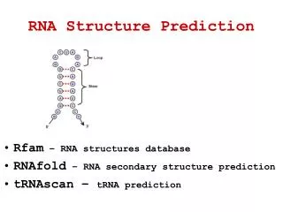
RNA Secondary Structure Prediction. Spring 2010. Objectives. Can we predict the structure of an RNA? Can we predict the structure of a protein?. RNA: Hypothesis and exclusions. Single stranded chain A RNA molecule is a string of n characters R=r 1 r 2 …r n such that r i {A,C,G,U}

E N D
RNA Secondary Structure Prediction Spring 2010
Objectives • Can we predict the structure of an RNA? • Can we predict the structure of a protein?
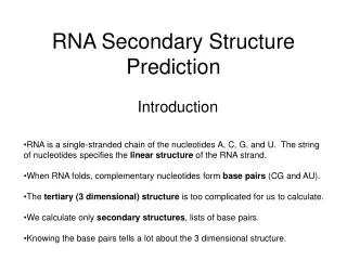
RNA: Hypothesis and exclusions • Single stranded chain • A RNA molecule is a string of n characters R=r1r2…rn such that ri {A,C,G,U} • Predicting methods are based on the computation of minimun free-energy configurations • We exclude the knots. • A knot exists when (ri, rj) S and (rk, rl) S and i<k<j<l.
Combinatorial Solution • Enumerate all the possible structures • Compute the one with the lowest free-energy • Impossible to solve: Exponential in the number of bases!
Independent Base Pair • Assumption: the energy of a base pair is independent of all the others. Let (ri,rj) be the free energy of base pair (ri, rj) • We assume that (ri,rj)=0 if i=j • We consider secondary structures and we use a dynamic programming approach
Dynamic programming • Consider the string Ri,j = R=riri+1…rj we want to compute the secondary structure Si,j of minimum energy Possible Cases: • rj is base-paired with ri • then E(Si,j) = (ri,rj) + E(Si,j-1) • rj does not pair with any base • then E(Si,j) = E(Si,j-1) • rj is base-paired with rk and ikj • then split the string in Ri,k-1 and Rk,j and • E(Si,j) = min{ E(Si,k-1) + E(Sk,j)}
The algorithm computes the matrix n x n using this minimization function Complexity of the algorithm: O(n3) O(n2) to compute the matrix times O(n) to compute each element of the matrix note that each element has a variable number of elements to consider that can be n in the worst case Dynamic Programming
Structures with loops • Assumption: the free energy of a base pair depends on adjacent base pairs A loop is a set of all bases accessible from a base pair (ri,rj) Consider (ri,rj) in S and positions u, v, and w such that i u v w j . We say that rv is accessible from (ri,rj), if (ru,rw) is not a base pair in S for any u and w
hairpin loop Loops bulge on i helical region interior loop
Dynamic programming • Determine Si,j forRi,j = R=riri+1…rj Possible Cases: • ri is not base-paired • then E(Si,j) = E(Si+1,j) • rj is not base-paired • then E(Si,j) = E(Si,j-1) • rj forms a pair with rk and ikj • split the string in Ri,k-1 and Rk,j and • then E(Si,j) = min { E(Si,k) + E(Sk+1,j) } • rj forms a pair with ri • that means that there might be one or more loops between i and j • E(Si,j) = E(Li,j)
The energy of a loop hairpin: • E(Li,j) = (ri,rj) + (j-i-1) • (k)=destabilizing free energy of hairpin loop of size k helical region: • E(Li,j) = (ri,rj) + + E(Si+1,j-1) • =stabilizing free energy of adjacent base pair bulge on i: • E(Li,j) = mink1{(ri,rj) + (k) + E(Si+k+1,j-1)} • (k) =destabilizing free energy of a bulge loop of size k bulge on j: • E(Li,j) = mink1{ (ri,rj) + (k) + E(Si+1,j-k-1)} interior loop: • E(Li,j) = mink1,k21{(ri,rj) + (k1+ k2) + E(Si+1,j-1)} • (k) =destabilizing free energy of a bulge loop of size K
Dynamic Programming E(Si+1,j) E(Si,j-1) E(Si,j) = min min{ E(Si,k) + E(Sk+1,j) } i<k<j E(Li,j) • Complexity of the algorithm: O(n4) • the complexity is worse because of the loops it takes constant time to compute the hairpin and helical region loop O(n2) • it takes linear time to compute the bulge since k ranges between 1 and j-i. O(n3) • it takes quadratic time to compute the interior loop since we are dealing with two parameters k1 and k2 therefore we have to look at a submatrix having O(n2) elements. O(n4)
CH3 Side Chain Alpha Carbon C H2N COOH Carboxy Group H Amino Group Protein Folding:Example Amino Acid
Protein Folding Problem Assumptionfor all protein folding prediction methods: amino acid sequence completely and uniquely determines the folding. Problem: Given the amino acid sequence of a protein, we would like to process it and determine where exactly the -helices, -sheets and loops are, and how they arrange themselves in motifs and domains
Combinatorial approach • Enumerate all the possible foldings, • compute the free energy of each • choose the one with minimum free energy
From what we know…. • if we assume that the angles and between the alpha carbon and the neighboring atoms assume only 3 possible values, we have that a protein with 100 residue has (32)100 possible configurations! • How do we compute the energy of a configuration? • factors: shape, size, polarity of the molecules, relative strenght of the interaction at molecular level, ect…too many factors and not a defined agreement • this problem applies to secondary structures as well. • What do we know? • hydrophobic amino acid stay "inside" the protein, hydrophillic amino acid stay "outside" the protein; • not enough information to make a prediction
Conclusions • No dynamic programming approach is know for protein secondary prediction • Programs based on neural nets to pattern-recognition based on statistical properties of residue in proteins are available • not as good as we desire. • new techniques must be developed • we discuss a branch and bound solution
Protein Threading Problem • Similar sequences should have similar structures • if A with a known protein structure, is similar to B at a sequence level, B structure should be nearly the same as A structure • Certain proteins are different at a sequence level but are structurally related, • ie. they have different kinds of loops but similar cores • Approach used for the solution: Branch and Bound
Core threading • Loops are structures that are neither helices nor -sheets • Protein Core are either helices and sheets • Motifs are simple combination of a few secondary structures (ex. helix-loop-helix)
Protein threading problem definition • Input: Given protein sequence A; Core structural model M; Score functions g1, g2. • Output:A threading T. In short: Align A to model T. • Given: • A: Protein sequence of length n: a1, a2, a3, … , an; • M: m core segments C1, C2, C3, … , Cm; • c1, c2, c3, … , cm; length of core segments; • l1, l2, l3, …, lm-1; loop regions connecting core segments; • l1max, l2max, l3max, …, lm-1max; maximum lengths of loop regions; • l1min, l2min, l3min, …, lm-1min; minimum lengths of loop regions; • Properties of each amino acid; • f, g1, g2: score functions to evaluate threading;
Output: T: t1, t2, t3, …, tm; start locations for core segments; score function where, g1 and g2 are based on the given model M. g1 shows how each segment corresponds to core segment i in the model, and g2 deals with the interactions between segments. So to solve the threading problem, we have to decide on t1, t2, t3, …, tm, so that the overall score is maximum. Thus the threading problem, or alignment problem, is converted to an optimization problem.
Threading constraints spacing constraint order of the core constraint
Branch and Bound • Assume we are minimizing f(s) and we aleady know the value f(s) for some candidate solutions in a set. • Branch • divide the solution space according to some constraints. For example, partition X in X1(all solutions having a certain property) and X2 (all solutions that do not) • Partition should be implicit, i.e. you do not explicitly enumerate the solutions • Bound • for every partition X, obtain a lower bound lb on the value of f(s) for every solution sX. • If f(s) < lb then we can discard all the candidate solutions in X because we have a solution, s, that scores better than all solutions in X, otherwise we explore the set X
Branch and Bound-Issues • Constructing score function • Calculating lower bound • Choosing split segment • Choosing split point
Protein Threading: Branch and Bound • Set of all possible threadings defined by initial position bounds • This implicitely defined by the number of aminoacids in A • Divide possible threadings into smaller sets, and compute new position bounds for each set • Compute a quick score lower bound for each set of threadings • Keep re-dividing the set with smallest lower bound, until set size if 1.
3. Compute the lower bound: Branch and Bound • Given a set of threadings defined by position bounds, one possible score lower bound is this is an approximation
10-20 0-100 250 10 5 0-100 1 206 266 476 6 101
80 32 35 (1…23) (24) (24...49) 50 80 34 (34…49) (25…29) (30) set of possible threadings: amino acids (1…100) 30 70 60 (1…49) (50) (51…100)