Download
1 / 22
220 likes | 375 Vues
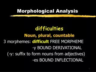
Co-Occurrence and Morphological Analysis for Colon Tissue Biopsy Classification. Khalid Masood, Nasir Rajpoot, Kashif Rajpoot*, Hammad Qureshi Signal and Image Processing Group, University of Warwick (UK) * Wolfson Medical Vision Lab, Oxford University (UK). Problem Definition.

E N D
Co-Occurrence and Morphological Analysis for Colon Tissue Biopsy Classification • Khalid Masood, Nasir Rajpoot, Kashif Rajpoot*, Hammad Qureshi • Signal and Image Processing Group, University of Warwick (UK) • * Wolfson Medical Vision Lab, Oxford University (UK)
Problem Definition • Given hyperspectral image cube of a patient’s colon tissue biopsy sample, automatically label the sample as Benign or Malignant Benign Malignant • Our approach is based on the idea that malignancy of a tumor alters the macro-architecture of the tissue glands: • Nice tubular structure of the glands for benign tumors • No such structure for malignant tumors
Motivation for Colon Biopsy Classification • Useful for screening of the colon cancer • Visual assessment by pathologists is very subjective • Significant intra- and inter-observational variation between pathologists • Quantitative histopathological analysis techniques offer objective, reliable, accurate, and reproducible assessment Source: NIH
Hyperspectral Imaging + Ordinary cameras only capture reflections from RGB colors Hyperspectral cameras capture reflections from a range of visible wavelengths
Hyperspectral Imaging (HSI) • HSI is a fast and reliable means of characterizing the histochemistry of tissues • HSI is also used extensively in remote sensing, satellite imaging, and defence (target detection etc.) applications • The Nuance multispectral imaging system can acquire 20 subbands in visible wavelength range of 420-720nm • Each hyperspectral image is a 3D data cube with a spectral coordinate in the z direction representing 20 subbands
Our Classification Algorithm • Based on a spectral-spatial analysis of the input data cube, our algorithm consists of three stages: • Stage I: Dimensionality reduction, followed by segmentation • Stage II: Morphological/textural analysis of the segmented results • Stage III: Classification using Subspace Projection methods and Support Vector Machines (SVM)
Stage I: Segmentation • Dimensionality reduction (from 20 to 4 bands of the multispectral image cube) is achieved using independent component analysis (ICA) and k-means clustering • Nuclei, cytoplasm; gland secretions;stroma of the lamina propria
Stage II: Feature Extraction • Four binary images are extracted from each segmented image • Two sets of features are calculated: morphological and co-occurrence matrix features: • Morphological Features: • These describe the shape, size, orientation and other attributes of the cellular components • These features are calculated on patches (blocks) of the segmented image • Co-Occurrence Features: • These describe the textural properties of a given neighborhood
Morphological Features • Morphological features describe the shape and texture of the image • Feature vector consists of five to ten morphological features • Discriminant morphological features are: • Euler Number : number of contiguous parts • Convex Area : number of pixels in convex image • Extent : the proportion of pixels in the bounding box • Solidity : the proportion of pixels in the convex hull • Area : the actual number of pixels in the patch • EquivDiameter : the diameter of a circle with the same area as of the patch
Co-occurrence Features • The co-occurrence matrix is constructed by analysing the gray levels of neighboring pixels • The (i,j)th element of a co-occurrence matrix for a particular angle and distance is given by the joint conditional pdf: • Three attributes used are:
Stage III : Classification • Subspace Projection methods • Principle Component Analysis (PCA) • Linear Discriminant Analysis (LDA) • Kernel PCA • Kernel LDA • Support Vector Machines (SVM) • Polynomial kernel • Gaussian kernel
Principal Component Analysis (PCA) • Eigenvectors of the data in the embedding space can be used to detect directions of maximum variance. • The principal components can be computed by solving the eigenvalue problem: • The coefficients of projection along a few top principal directions can be used as features • Nearest-neighbor classifier is used for assigning label to a biopsy sample
Linear Discriminant Analysis (LDA) • Limitations of the PCA • As opposed to PCA, which maximises the overall scatter, LDA maximises the ratio of between-class scatter Sb to within-class scatter Sw • The wi can be computed by solving the generalised eigenvalue problem:
Linear Boundary Assumption • In most real-world problems, separating boundaries are not necessarily linear! Consider, for instance, the following example: Will a linear classifier work?
The Kernel Trick • Kernel machines (eg, SVMs) transform non-linear decision boundaries to linear ones in higher dimensional feature space • Two dimensional features (let us say) are mapped to a three dimensional feature space through a non-linear transform • Non-linear ellipsoidal decision boundary is replaced to linear boundary in higher dimensional space • The trick is to replace dot products in F with a kernel function in the input space R so that the non-linear mapping is performed implicitly in R
SVM Kernel Functions • A few commonly used kernel functions are: • Classifier’s performance highly sensitive to parameter values • Best kernel parameter values are searched
Experimentation • Two sets of Experiments: Mixed testing and Leave one out (LOO) • For mixed testing: • 4096 patches (blocks) per image of 16x16 dimensions per patch • Morphological features • Training set contains one quarter of the patches while remaining three quarters make the test set • PCA and modular LDA are used in mixed testing • Leave one out testing is done on gray level co-occurrence features • 16x16 patches • Support Vector Machines (polynomial kernel and gaussian kernel are used) • Kernel parameters are optimized • Classification label is assigned to a slide according to the class of the majority of the patches
Experimental Results • AUCH of the ROC curve for LDA goes up to 0.92 for 5 features.
Conclusions and Future Work • Conclusions • Tissue segmentation affects the performance • Implementation of LDA saves the computational cost and the performance achieved by it is encouraging • Gaussian kernel SVM gives no false alarm • Future Work • More effective segmentation • Combination of classifiers • Shape modelling of nuclei glands
Acknowledgements • Prof David Rimm, Department of Pathology, Yale University School of Medicine (USA) • Prof Gustave Davis, Department of Pathology, Yale University School of Medicine (USA) • Prof Ronald Coifman, Department of Applied Mathematics, Yale University (USA)
Thanks for your attention Any Questions?