Download
1 / 29
300 likes | 449 Vues
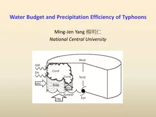
On the Definition of Precipitation Efficiency. Sui, C.-H., X. Li, and M.-J. Yang, 2007: On the definition of precipitation efficiency. J. Atmos. Sci. , 64 , 4506–4513. Professor : Ming-Jen Yang Student : Yi-Chuan Chung Date : 2013/11/15. Introduction.

E N D
On the Definition of Precipitation Efficiency Sui, C.-H., X. Li,and M.-J. Yang, 2007:On the definition of precipitation efficiency. J. Atmos. Sci., 64, 4506–4513. Professor : Ming-Jen Yang Student: Yi-Chuan Chung Date : 2013/11/15
Introduction • Precipitationis directly produced by cloud microphysics processes at convective temporal and spatial scales. But the occurrence of precipitation is associated with environmental dynamics and thermodynamicsof weather and climate events. • So precipitation can be simply assumed to be proportional to the condensation rate (microphysical view) or the moisture flux in the convective systems (large-scale view). • Due to reevaporationof rain and local atmospheric moistening, not all condensation or moisture fluxes are used to produce precipitation. Therefore, precipitation efficiency is defined to evaluate how efficiently the convective system produces precipitation.
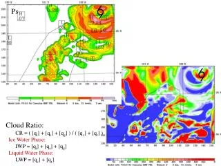
Introduction • CMPE(CloudMicrophysicsPrecipitationEfficiency): The ratio of the surface rain rate to the sum of vapor condensation and deposition rates. • LSPE (Large-ScalePrecipitation Efficiency): Theratio of the surface rain rate to the sum of vapor convergenceand surface evaporation rates. CMPE L
Introduction Precipitation efficiency remains to bedefined properly and to becalculated accurately. • Both LSPE and CMPE could be greater than 100% • LSPE could be negative What causes these physically unreasonable precipitation efficiencies? How should precipitation efficiency be defined and calculated properly?
Model setup • The two-dimensionalcloud-resolving model simulation data during the Tropical Ocean Global Atmosphere Coupled Ocean– Atmosphere Response Experiment (TOGA COARE). • The horizontal boundary is periodic. • The horizontal domain is 768 km with a grid resolution of 1.5 km. • The vertical grid resolution ranges from about 200 m near the surface to about 1 km near 100 mb. Z 100 mb X 768 km
Model setup • The model is integrated from 0400local standard time (LST) 18 December 1992to 1000 LST 9 January 1993 (21.25 days total). • The time step is 12 s. • Time evolution of the • vertical distribution of the large-scale vertical velocity and zonal wind. • The time series of the SST. • which are imposed in the • model during the integrations. • Hourly96-km-mean simulation data are used in the following analysis .
Method a. [ ] : Denotes a vertically integrated quantity b. sgn( )
CMPE Hydrometeor budget equation C = qc + qr + qi + qs + qg :Local hydrometeor change : Hydrometeor convergence : Surface precipitation : Sink term in the water vapor budget = [PCND]+[PDEP] + [PSDEP] + [PGDEP] Cloud water Snow Cloud ice Graupel : Source term in the water vapor budget = [REVP]+[MLTG] + [MLTS] Graupel Rain Snow
CMPE • Cloud microphysics precipitation efficiency Sui et al. (2005)
CMPE CMPE1 (%) vsCMPE2 (%) using hourly 96-km averaged data during the 21-day integration. CMPE1 ranges from 0% to 350% CMPE2 is between 0% and 100%
CMPE CMPE1 and CMPE2vsPs • Both CMPE1 and CMPE2 have • a tendency to converge to a • finite value as Ps increases For strong rainfall (Ps>5 mm/ hr) Both CMPE1 and CMPE2 range from 50% to 100%. For weak rainfall (Ps < 5 mm/ hr) CMPE1 ranges from 0% to 350%. • CMPE1 is sensitive to rainfall • sources QCM during light rains.
LSPE • water vapor budget : Local vapor change : Vapor convergence : Surface evaporation rate : Sink term in the water vapor budget : Source term in the water vapor budget
LSPE • water vapor budget • Hydrometeor budget equation : Local vapor change : Vapor convergence : Sum of local hydrometeor change and hydrometeor convergence : Surface evaporation rate
LSPE • Large-scale precipitation efficiency Sui et al. (2005)
LSPE LSPE1 (%) vsLSPE2 (%) using hourly 96-km averaged data during the 21-day integration. LSPE1 ranges from -500% to 500% LSPE2 ranges between 0% and 100%
LSPE LSPE1 and LSPE2 as functions of Ps • LSPE2tends to increase with increasing Ps such that the range of LSPE2 narrows with increasing Ps. • LSPE1have a much wider range and converge to a finite value with increasing Ps. • Negative values of LSPE1 correspond to weak rainfall condition (Ps < 5 mm/ hr).
LSPE • Large-scale precipitation efficiency
LSPE LSPE2 is calculated by setting QCM to be zero [LSPE2(QCM=0)] LSPE2(QCM=0)vsLSPE2 • LSPE2(QCM=0) is generally larger than LSPE2, and could be larger than 100%, especially when LSPE2 is larger .
CMPE2vsLSPE2 using hourly 96-km averaged data during the 21-day integration. • The RMSdifference between CMPE2 and LSPE2 is 18.5%, smaller than the standard deviations of CMPE2 (28.5%) and LSPE2 (35.1%). • The linearcorrelation coefficient between CMPE2 and LSPE2 is 0.85
CMPE2vsLSPE2 To examine the dependence of PE on temporal and spatial scales. The linear correlation coefficient decreases and RMSdifference increases as the time period of averaged data increases.
CMPE2vsLSPE2 • Spatial scales of averaged data (a) Hourly 48-kmaveraged (b) Hourly 24-km averaged LSPE2 and CMPE2 are insensitive to spatial scales of averaged data.
CMPE2vsLSPE2 • Time period of averaged data (b) Dailymean 96-km averaged (a) 6-hourlymean 96-km averaged LSPE2 is largerthan CMPE2 for higher values of precipitation efficiency, whereas it is the opposite for lower values of precipitation efficiency. LSPE2 is largerthan CMPE2 for higher values of precipitation efficiency, whereas it is the opposite for lower values of precipitation efficiency.
Summery • Simplified precipitation efficiencies like LSPE1and CMPE1may be larger than 100% when some source terms are excluded in the calculations. This is more likely to occur in the light rain conditions. • More complete definitions of precipitation efficiency are proposed in this study based on either the moisture budget (LSPE2) or hydrometeor budget (CMPE2) that include all sources related to surface rainfall processes. 1. LSPE2 and CMPE2 range from 0% to 100% . 2. LSPE2 and CMPE2 are highly correlated. (We shall demonstrate that despite different aspects, LSPE and CMPE are fundamentally the same based on physical considerations.) 3. Their linear correlation coefficient and root-mean-squared difference are moderately sensitive to the time period of averaged data, whereas they are not sensitive to the spatial scales of averaged data. • CMPE2 (or CMPE1) is a physically more straightforward definition of precipitation efficiency than LSPE2(or LSPE1). • Butthe former can only be estimated in models with explicit parameterization of cloud microphysics, which is model-dependent, while the latter may be estimated based on currently available assimilation data of satellite and sounding measurements.
Microphysics parameterizations in the cloud-resolv-ing model used in this study are based on the schemes proposed by Rutledge and Hobbs (1983, 1984; hereafter RH83 and RH84,) Lin et al. (1983, LFO), Tao et al.(1989, TSM), Hsie et al. (1980, HFO), and Krueger et al. (1995, KFLC), respectively.
Model setup • The two-dimensionalcloud-resolving model simulation data during the Tropical Ocean Global Atmosphere Coupled Ocean– Atmosphere Response Experiment (TOGA COARE). • The horizontal boundary is periodic. • The horizontal domain is 768 km with a grid resolution of 1.5 km. • The vertical grid resolution ranges from about 200 m near the surface to about 1 km near 100 mb. • The time step is 12 s. • Hourly 96-km-mean simulation data are used in the following analysis .
LSPE • water vapor budget • Hydrometeor budget equation : Vapor convergence : Local vapor change : Sum of local hydrometeor change and hydrometeor convergence : Surface evaporation rate
LSPE LSPE2 is calculated by setting QCM to be zero [LSPE2(QCM=0)] LSPE2(QCM=0)vsLSPE2 • LSPE2(QCM=0) is generally larger than LSPE2, and could be larger than 100%, especially when LSPE2 is larger . • LSPE2 could be a strong function of both water vapor and cloud hydrometeors, though it ranges between 0% and 100%. • This suggests that CMPE may be a more appropriate parameter for the estimation of precipitation efficiency in cloud models.