Download
1 / 37
430 likes | 500 Vues
Logistic Regression. Logistic Regression - Dichotomous Response variable and numeric and/or categorical explanatory variable(s) Goal: Model the probability of a particular as a function of the predictor variable(s) Problem: Probabilities are bounded between 0 and 1

E N D
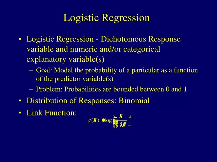
Logistic Regression • Logistic Regression - Dichotomous Response variable and numeric and/or categorical explanatory variable(s) • Goal: Model the probability of a particular as a function of the predictor variable(s) • Problem: Probabilities are bounded between 0 and 1 • Distribution of Responses: Binomial • Link Function:
Logistic Regression with 1 Predictor • Response - Presence/Absence of characteristic • Predictor - Numeric variable observed for each case • Model - p(x) Probability of presence at predictor level x • b = 0 P(Presence) is the same at each level of x • b > 0 P(Presence) increases as x increases • b < 0 P(Presence) decreases as x increases
Logistic Regression with 1 Predictor • a, b areunknown parameters and must be estimated using statistical software such as SPSS, SAS, or STATA • Primary interest in estimating and testing hypotheses regarding b • Large-Sample test (Wald Test): • H0: b = 0 HA: b 0
Example - Rizatriptan for Migraine • Response - Complete Pain Relief at 2 hours (Yes/No) • Predictor - Dose (mg): Placebo (0),2.5,5,10
Odds Ratio • Interpretation of Regression Coefficient (b): • In linear regression, the slope coefficient is the change in the mean response as x increases by 1 unit • In logistic regression, we can show that: • Thus ebrepresents the change in the odds of the outcome (multiplicatively) by increasing x by 1 unit • If b = 0, the odds and probability are the same at all x levels (eb=1) • If b > 0 , the odds and probability increase as x increases (eb>1) • If b < 0 , the odds and probability decrease as x increases (eb<1)
95% Confidence Interval for Odds Ratio • Step 1: Construct a 95% CI for b : • Step 2: Raise e = 2.718 to the lower and upper bounds of the CI: • If entire interval is above 1, conclude positive association • If entire interval is below 1, conclude negative association • If interval contains 1, cannot conclude there is an association
Example - Rizatriptan for Migraine • 95% CI for b : • 95% CI for population odds ratio: • Conclude positive association between dose and probability of complete relief
Multiple Logistic Regression • Extension to more than one predictor variable (either numeric or dummy variables). • With k predictors, the model is written: • Adjusted Odds ratio for raising xi by 1 unit, holding all other predictors constant: • Many models have nominal/ordinal predictors, and widely make use of dummy variables
Testing Regression Coefficients • Testing the overall model: • L0, L1 are values of the maximized likelihood function, computed by statistical software packages. This logic can also be used to compare full and reduced models based on subsets of predictors. Testing for individual terms is done as in model with a single predictor.
Example - ED in Older Dutch Men • Response: Presence/Absence of ED (n=1688) • Predictors: (p=12) • Age stratum (50-54*, 55-59, 60-64, 65-69, 70-78) • Smoking status (Nonsmoker*, Smoker) • BMI stratum (<25*, 25-30, >30) • Lower urinary tract symptoms (None*, Mild, Moderate, Severe) • Under treatment for cardiac symptoms (No*, Yes) • Under treatment for COPD (No*, Yes) * Baseline group for dummy variables
Example - ED in Older Dutch Men • Interpretations: Risk of ED appears to be: • Increasing with age, BMI, and LUTS strata • Higher among smokers • Higher among men being treated for cardiac or COPD
Loglinear Models with Categorical Variables • Logistic regression models when there is a clear response variable (Y), and a set of predictor variables (X1,...,Xk) • In some situations, the variables are all responses, and there are no clear dependent and independent variables • Loglinear models are to correlation analysis as logistic regression is to ordinary linear regression
Loglinear Models • Example: 3 variables (X,Y,Z) each with 2 levels • Can be set up in a 2x2x2 contingency table • Hierarchy of Models: • All variables are conditionally independent • Two of the pairs of variables are conditionally independent • One of the pairs are conditionally independent • No pairs are conditionally independent, but each association is constant across levels of third variable (no interaction or homogeneous association) • All pairs are associated, and associations differ among levels of third variable
Loglinear Models • To determine associations, must have a measure: the odds ratio (OR) • Odds Ratios take on the value 1 if there is no association • Loglinear models make use of regressions with coefficients being exponents. Thus, tests of whether odds ratios are 1, is equivalently to testing whether regression coefficients are 0 (as in logistic regression) • For a given partial table, OR=eb, software packages estimate and test whether b=0
Example - Feminine Traits/Behavior • 3 Variables, each at 2 levels (Table contains observed counts): • Feminine Personality Trait (Modern/Traditional) • Female Role Behavior (Modern/Traditional) • Class (Lower Classman/Upper Classman)
Example - Feminine Traits/Behavior • Expected cell counts under model that allows for association among all pairs of variables, but no interaction (association between personality and role is same for each class, etc). Model:(PR,PC,RC) • Evidence of personality/role association (see odds ratios) Note that under the no interaction model, the odds ratios measuring the personality/role association is same for each class
Example - Feminine Traits/Behavior • Intuitive Results: • Controlling for class in school, there is an association between personality trait and role behavior (ORLower=ORUpper=3.88) • Controlling for role behavior there is no association between personality trait and class (ORModern= ORTraditional=1.06) • Controlling for personality trait, there is no association between role behavior and class (ORModern= ORTraditional=1.12)
SPSS Output • Statistical software packages fit regression type models, where the regression coefficients for each model term are the log of the odds ratio for that term, so that the estimated odds ratio is e raised to the power of the regression coefficient. Parameter Estimates Asymptotic 95% CI Parameter Estimate SE Z-value Lower Upper Constant 3.5234 .1651 21.35 3.20 3.85 Class .4674 .2050 2.28 .07 .87 Personality -.8774 .2726 -3.22 -1.41 -.34 Role -1.1166 .2873 -3.89 -1.68 -.55 C*P .0605 .3064 .20 -.54 .66 C*R .1166 .3107 .38 -.49 .73 R*P 1.3554 .2987 4.54 .77 1.94 Note: e1.3554 = 3.88 e.0605 = 1.06 e.1166 = 1.12
Interpreting Coefficients • The regression coefficients for each variable corresponds to the lowest level (in alphanumeric ordering of symbols). Computer output will print a “mapping” of coefficients to variable levels. To obtain the expected cell counts, add the constant (3.5234) to each of the bs for that row, and raise e to the power of that sum
Goodness of Fit Statistics • For any logit or loglinear model, we will have contingency tables of observed (fo) and expected (fe) cell counts under the model being fit. • Two statistics are used to test whether a model is appropriate: the Pearson chi-square statistic and the likelihood ratio (aka Deviance) statistic
Goodness of Fit Tests • Null hypothesis: The current model is appropriate • Alternative hypothesis: Model is more complex • Degrees of Freedom: Number of sample logits-Number of parameters in model • Distribution of Goodness of Fit statistics under the null hypothesis is chi-square with degrees of freedom given above • Statistical software packages will print these statistics and P-values.
Example - Feminine Traits/Behavior Table Information Observed Expected Factor Value Count % Count % PRSNALTY Modern ROLEBHVR Modern CLASS1 Lower Classman 33.00 ( 15.79) 34.10 ( 16.32) CLASS1 Upper Classman 19.00 ( 9.09) 17.90 ( 8.57) ROLEBHVR Traditional CLASS1 Lower Classman 25.00 ( 11.96) 23.90 ( 11.44) CLASS1 Upper Classman 13.00 ( 6.22) 14.10 ( 6.75) PRSNALTY Traditional ROLEBHVR Modern CLASS1 Lower Classman 21.00 ( 10.05) 19.90 ( 9.52) CLASS1 Upper Classman 10.00 ( 4.78) 11.10 ( 5.31) ROLEBHVR Traditional CLASS1 Lower Classman 53.00 ( 25.36) 54.10 ( 25.88) CLASS1 Upper Classman 35.00 ( 16.75) 33.90 ( 16.22) Goodness-of-fit Statistics Chi-Square DF Sig. Likelihood Ratio .4695 1 .4932 Pearson .4664 1 .4946
Example - Feminine Traits/Behavior Goodness of fit statistics/tests for all possible models: The simplest model for which we fail to reject the null hypothesis that the model is adequate is: (C,PR): Personality and Role are the only associated pair.
Adjusted Residuals • Standardized differences between actual and expected counts (fo-fe, divided by its standard error). • Large adjusted residuals (bigger than 3 in absolute value, is a conservative rule of thumb) are cells that show lack of fit of current model • Software packages will print these for logit and loglinear models
Example - Feminine Traits/Behavior • Adjusted residuals for (C,P,R) model of all pairs being conditionally independent: Adj. Factor Value Resid. Resid. PRSNALTY Modern ROLEBHVR Modern CLASS1 Lower Classman 10.43 3.04** CLASS1 Upper Classman 5.83 1.99 ROLEBHVR Traditional CLASS1 Lower Classman -9.27 -2.46 CLASS1 Upper Classman -6.99 -2.11 PRSNALTY Traditional ROLEBHVR Modern CLASS1 Lower Classman -8.85 -2.42 CLASS1 Upper Classman -7.41 -2.32 ROLEBHVR Traditional CLASS1 Lower Classman 7.69 1.93 CLASS1 Upper Classman 8.57 2.41
Comparing Models with G2 Statistic • Comparing a series of models that increase in complexity. • Take the difference in the deviance (G2) for the models (less complex model minus more complex model) • Take the difference in degrees of freedom for the models • Under hypothesis that less complex (reduced) model is adequate, difference follows chi-square distribution
Example - Feminine Traits/Behavior • Comparing a model where only Personality and Role are associated (Reduced Model) with the model where all pairs are associated with no interaction (Full Model). • Reduced Model (C,PR): G2=.7232, df=3 • Full Model (CP,CR,PR): G2=.4695, df=1 • Difference: .7232-.4695=.2537, df=3-1=2 • Critical value (a=0.05): 5.99 • Conclude Reduced Model is adequate
Logit Models for Ordinal Responses • Response variable is ordinal (categorical with natural ordering) • Predictor variable(s) can be numeric or qualitative (dummy variables) • Labeling the ordinal categories from 1 (lowest level) to c (highest), can obtain the cumulative probabilities:
Logistic Regression for Ordinal Response • The odds of falling in category j or below: • Logit (log odds) of cumulative probabilities are modeled as linear functions of predictor variable(s): This is called the proportional odds model, and assumes the effect of X is the same for each cumulative probability
Example - Urban Renewal Attitudes • Response: Attitude toward urban renewal project (Negative (Y=1), Moderate (Y=2), Positive (Y=3)) • Predictor Variable: Respondent’s Race (White, Nonwhite) • Contingency Table:
SPSS Output • Note that SPSS fits the model in the following form: Note that the race variable is not significant (or even close).
Fitted Equation • The fitted equation for each group/category: For each group, the fitted probability of falling in that set of categories is eL/(1+eL) where L is the logit value (0.264,0.264,0.541,0.541)
Inference for Regression Coefficients • If b = 0, the response (Y) is independent of X • Z-test can be conducted to test this (estimate divided by its standard error) • Most software will conduct the Wald test, with the statistic being the z-statistic squared, which has a chi-squared distribution with 1 degree of freedom under the null hypothesis • Odds ratio of increasing X by 1 unit and its confidence interval are obtained by raising e to the power of the regression coefficient and its upper and lower bounds
Example - Urban Renewal Attitudes • Z-statistic for testing for race differences: Z=0.001/0.133 = 0.0075 (recall model estimates -b) • Wald statistic: .000 (P-value=.993) • Estimated odds ratio: e.001 = 1.001 • 95% Confidence Interval: (e-.260,e.263)=(0.771,1.301) • Interval contains 1, odds of being in a given category or below is same for whites as nonwhites
Ordinal Predictors • Creating dummy variables for ordinal categories treats them as if nominal • To make an ordinal variable, create a new variable X that models the levels of the ordinal variable • Setting depends on assignment of levels (simplest form is to let X=1,...,c for the categories which treats levels as being equally spaced)