Download
1 / 25
250 likes | 280 Vues
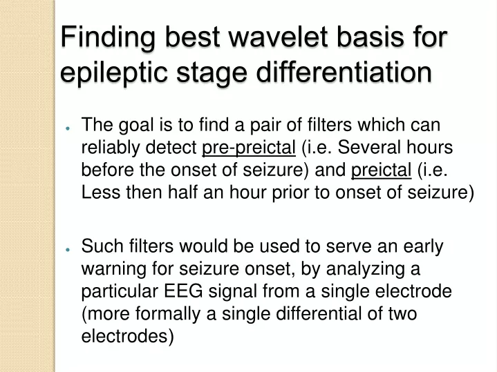
Finding best wavelet basis for epileptic stage differentiation. The goal is to find a pair of filters which can reliably detect pre-preictal (i.e. Several hours before the onset of seizure) and preictal (i.e. Less then half an hour prior to onset of seizure (

E N D
Finding best wavelet basis for epileptic stage differentiation The goal is to find a pair of filters which can reliably detect pre-preictal (i.e. Several hours before the onset of seizure) and preictal (i.e. Less then half an hour prior to onset of seizure( Such filters would be used to serve an early warning for seizure onset, by analyzing a particular EEG signal from a single electrode (more formally a single differential of two electrodes(
Signal analysis – background Several methods exist for detecting features in discrete signal. One such method is a Fourier transform, in particular the DFT (Discrete Fourier Transform), which has an efficient numeric implementation known as FFT (Fast Fourier Transform) Another widespread family of transforms are wavelet transforms.
Transforms temporal signal representationinto frequency domain – each ”finite-power” signal can be represented as a linear combination of scalings of sine and cosine functions. Those scalings correspond to the different frequencies. Fourier transform
Fourier – example Fourier (only real part)
Fourier transform - limitations Provides no temporal localization of detected features. (i.e. If the function has a discontinuity it is possible to see it in the frequency domain, however it is impossible to deduce where is it in the time domain) Gibb's phenomena – the inability to precisely describe discontinuous functions: for instance the following are approximations for square wave: 5 approx. steps 125 approx. Steps. The maximal difference is still the same (non-uniform convergence) 25 approx. steps
Wavelet transforms A family of transforms based on the notion of a scaling function and a wavelet function, from which the basis of L2(R) is ultimately derived. (by scaling and shifting the wavelet function) Another way to look at the tranform is from the point of view of MRA. (Multi-resolution analysis)
Wavelets - MRA The wavelet basis can also be derived from two following recurrences: These are relations which define the scaling and the wavelet function, respectively. In fact it can be proven that these functions can be uniquely derived from {hk} and {gl}. If these sets furthermore satisfy certain conditions then the result is an orthogonal basis.
Wavelets – cont. If the {hk} and {gl} are finite, then we have wavelets with finite support. Those allow for simpler numerical computations
Wavelets vs. Fourier analysis Wavelets allow the inspection of local behaviours of a signal. (this is because each wavelet coefficient is affected only by a finite support, depending on the scale) Wavelets allow for MRA – localizing the analysis if required, or looking at more general properties of a signal as Fourier does. Wavelets allow building arbitrary level (subject to scale limitations) of ”approximation” of the signal between the most crude (expressed by only scaling-coefficients) and the most accurate (the signal itself, represented by full dyadic decomposition)
Wavelets vs. Fourier analysis Wavelets allow one to inspect only fixed set of frequencies (scales) if dyadic decomposition is used or result in excessive information (doubling the dimension!) if continuous wavelet transform is used. There are plenty of compromises between these two approaches, though. (We limit ourselves here to orthonormal wavelet bases, though there are transform variations which do not require orthonormality)
Entropy In information theory , entropy is a measure of the uncertainty associated with random variable.The entropy rate of a data source means the average number of bits per symbol needed to encode it p denotes the probability mass function of X I(X) is the information content
Entropy based best basis The best basis algorithm purpose is to select the most ”meaningful” basis for a signal representation. That, a set of filters such as the resulting coefficient convey real information, and not stay fixed during the whole signal duration. (The most ”informative” signal according to the entropy function is one whose coefficients are distributed uniformly across temporal shifts of the signal)
Tree of orthonormal bases 1.Subset of basis vectors can be identified with intervals of N of form 2.Each basis in the library corresponds to a disjoint cover of N by intervals 3.If is the subspace identified with Then
Selecting the best basis Orthonormal tree search for best basis by induction . Donate Bn,k the basis of signal corresponding to Ink , and An,k the best basis for the same interval, For K=0 ther is single basis (An,0 = Bn,0). For K>0, *E – entropy , but can be any additive cost function
Code example function [ output_args ] = sd1( input_args ) %SD1 find best basis coefficent, find and print best basis tree % gnerate best basis from 50% overlapping windows of size s signal=input_args; s=2048; %define window size 2^(k), k =1,2,3.... count=0; mean_coff_tree= zeros(s,log2(s)+1); %run over 50% overlapping window and sum cofficent while length(signal)>(s-1) cur_window=signal(1:s); signal=signal((s/2+1):length(signal)); %get cofficent for single window cof_tree=find_coff(cur_window); mean_coff_tree=mean_coff_tree+cof_tree; count=count+1 end %calculate mean of output_args=mean_coff_tree./count; titlestr = 'test'; D=log2(s); %Build tree with entropy numbers output_args= CalcStatTree(output_args,'Entropy'); [btree,vtree] = BestBasis(output_args,D); signaltitle = [' CP Best Basis; ' titlestr]; hold on PlotBasisTree(btree,D,output_args,signaltitle); xlabel('Splits of Time Domain') ylabel('Entropy Drop') return function [ output_args ] = find_coff( input_args ) %FIND_COFF find cofficet of input D=log2(length(input_args)); %Generate Orthonormal QMF (quadrature mirror filter) %for Wavelet Transform qmf = MakeONFilter('Haar'); %output array of Wavelet Packet Decompositions %Coefficients for frequency interval % [b/2^d,(b+1)/2^d] is stored in wp(packet(d,b,n),d+1) cof_tree=WPAnalysis(input_args,D,qmf); output_args=cof_tree return
Function usage for very short signal signal = [3 4 6 6 4 4 1 1] %Generate Orthonormal QMF (quadrature mirror filter) %for Wavelet Transform Input>> qmf = MakeONFilter('Haar') output>> qmf = 0.7071 0.7071 %output array of Wavelet Packet Decompositions %Coefficients for frequency interval % [b/2^d,(b+1)/2^d] is stored in wp(packet(d,b,n),d+1) Input>> cof_tree=WPAnalysis(pre1,3,qmf) Output>> cof_tree = 3.0000 4.9497 9.5000 10.2530 4.0000 8.4853 5.0000 -3.1820 6.0000 5.6569 2.5000 -3.8891 6.0000 1.4142 -3.0000 -0.3536 4.0000 0.7071 -0.5000 -0.3536 4.0000 0 0 0.3536 1.0000 0 0.5000 -0.3536 1.0000 0 0 0.3536 %Build tree with entropy numbers Input>> entrophy_val=CalcStatTree(cof_tree,'Entropy') Output >> entrophy_val = Columns 1 through 5 1.7388 1.0507 0.0213 0.5728 0.3291 Columns 6 through 10 0.0119 0.0119 0.1766 0.1979 0.2493 Columns 11 through 15 0.0066 0.0066 0.0066 0.0066 0.0066 Relatet to 1 depth decomposion Relatet to 2 depth decomposion Relatet to 3 depth decomposion Relatet to 4 depth decomposion
Short signal - First step example Origin signal D1 coefficients D2 coefficients D3 coefficients D4 coefficients ***Numbers upon subsets are correlated entropy values
Best basis for 2048 samples length signal function [ output_args ] = OneWin( input_args ) %finding the best basis tree for one window subj= load('Subject1/subj1_data_seizure1'); p_pre=subj.pre_preictal; p_pre1=p_pre(1,:); n = length(p_pre1) t = (0:(n-1))./n; figure; subplot(3,1,1); plot(t,p_pre1); title('pre_preictal full signal'); w_size=2048; n=w_size; t = (0:(n-1))./n; D=log2(w_size) subplot(3,1,2); plot(t,p_pre1(1:w_size)); title('pre_preictal first window of size 2048'); qmf = MakeONFilter('Haar'); cof_tree=WPAnalysis(p_pre1(1:w_size),D,qmf); output_args= CalcStatTree(cof_tree,'Entropy'); [btree,vtree] = BestBasis(output_args,D); subplot(3,1,3); signaltitle = ['first window']; PlotBasisTree(btree,D,output_args,signaltitle); return end
Step by step (middle step) Step 1. The signal Step 2. Find coeffients for all decomposition Step 3. Find best basis The relation for this resoulation can be clearly seen,For right side of the signal high level decomposition hold more information
Finding the mean coefficients (start) Find all decomposions Coeffients for each of the 50% overlap window separately
Finding the mean coefficients (cont) • To find mean derived best basis, we run over 50% overlapping windows , for each window, find stat tree and add it to the sum tree, also we count number of windows included. • At the end off the this process we divide each of the n*logn coefficient with the counter and we got mean coefficients tree. • To find std tree, we run over the signal for the second time , again find stat tree for each window, and use the mean coefficients we already got to find std for each one of the n*logncoffcients. see code at next two slides
Best Basis mean Derived (cont’) Generate mean coefficients for each decomposition mean_coff_tree= zeros(s,log2(s)+1); %run over 50% overlapping window and sum cofficent while length(signal)>(s-1) cur_window=signal(1:s); signal=signal((s/2+1):length(signal)); %get n*logn coefficient for single window cof_tree=find_coff(cur_window); %get n*logn sums of cofficents mean_coff_tree=mean_coff_tree+cof_tree; count=count+1 end %calculate mean of mean_coff_tree=mean_coff_tree./count; %get best basis for the mean coefficient m_stat_tree=CalcStatTree(mean_coff_tree,'Entropy'); [btree,vtree] = BestBasis(m_stat_tree,D); Fined best basis tree for mean coefficients
Find STD tree count=0; std_coff_tree= zeros(s,log2(s)+1); %run over 50% overlapping window and sum cofficent while length(signal)>(s-1) cur_window=signal(1:s); signal=signal((s/2+1):length(signal)); %get n*logn coefficient for single window cof_tree=find_coff(cur_window); %get n*logn of squr diff for single window std_tree=(cof_tree-m_cof_tree).^2; %get n*logn sums of squr diff std_coff_tree=std_coff_tree+std_tree; count=count+1; end %calc n*logn std std_coff_tree=sqrt(std_coff_tree/count)
Using WAVELAB 850 • A partial list of the techniques made available: • orthogonal and biorthogonal wavelet transforms, • translation-invariant wavelets, • interpolating wavelet transforms, • cosine packets, • wavelet packets, • matching pursuit, • Library used for first part • Wavelab850\Orthogonal library • routines in this directory perform periodic- and boundary-corrected wavelet analysis of 1-d and 2-d signals. • Wavelab850\Packets\One-D library • routines in this directory perform wavelet packet analysis and cosine packet analysis of 1-d signals.