Download
1 / 72
740 likes | 766 Vues
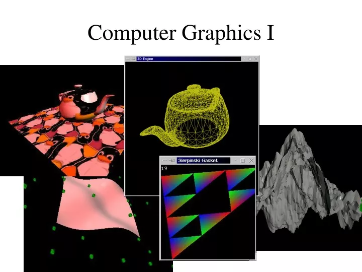
Computer Graphics I. Images in a computer. 94 100 104 119 125 136 143 153 157 158 103 104 106 98 103 119 141 155 159 160 109 136 136 123 95 78 117 149 155 160 110 130 144 149 129 78 97 151 161 158 109 137 178 167 119 78 101 185 188 161 100 143 167 134 87 85 134 216 209 172

E N D
Images in a computer... 94 100 104 119 125 136 143 153 157 158 103 104 106 98 103 119 141 155 159 160 109 136 136 123 95 78 117 149 155 160 110 130 144 149 129 78 97 151 161 158 109 137 178 167 119 78 101 185 188 161 100 143 167 134 87 85 134 216 209 172 104 123 166 161 155 160 205 229 218 181 125 131 172 179 180 208 238 237 228 200 131 148 172 175 188 228 239 238 228 206 161 169 162 163 193 228 230 237 220 199 … just a large array of numbers
True-color frame buffer Store R,G,B values directly in the frame-buffer. Each pixel requires at least 3 bytes => 2^24 colors.
Indexed-color frame buffer Store index into a color map in the frame-buffer. Each pixel requires at least 1 bytes => 2^8 simultaneous colors. Enables color-map animations.
Line algorithm 5, BresenhamBrushing up things a little Xdifference = (Xend-Xstart)Ydifference = (Yend-Ystart)Yerror = 2*Ydifference - XdifferenceStepEast = 2*YdifferenceStepNorthEast = 2*Ydifference - 2*Xdifferenceplot_pixel(x, y)loop x Xstart to Xend if Yerror <= 0 then Yerror = Yerror + StepEast else y = y + 1 Yerror = Yerror + StepNorthEast end_if plot_pixel(x, y)end_of_loop x Uses only integer maths => Fast!
Drawing polygons We draw our polygons scan line by scan line. This is called scan conversion. The process is done by following the edges of the polygon, and then fill between the edges.
Bi-linear interpolation Linear interpolation in two directions. First we interpolate in the y-direction, then we interpolate in the x-direction. Unique solution for flat objects (triangles are always flat.)
Anti-aliasing • Due to the discrete nature of our computers, aliasing effects appear in many situations, when drawing edges, shaded surfaces, textures etc. To reduce the effect of aliasing various anti-aliasing techniques can be applied. Some examples are: • Low-pass filtering (poor mans anti-aliasing) • Area-sampling (colour proportional to area) • Super-sampling (more samples than pixels) • Dithering (anti-aliasing in the colour domain) • MIP mapping (prefiltering for textures)
COLOR Color = The eye’s and the brain’s impression of electromagnetic radiation in the visual spectra. How is color perceived? detector rods & cones light source red-sensitive green-sensitive blue-sensitive reflecting object
The Fovea There are three types of cones, S, M and L
standard lightsource object reflectance CIE 1931 standard observer CIE XYZ values z X=14.27 Y=14.31 Z=71.52 x y x x = 400nm 700nm 400nm 700nm 400nm 700nm Each color is represented by a point (X,Y,Z) in the 3D CIE color space. The point is called the tristimulus value.
Projection of the CIE XYZ-space Perceptual equal distances
Mixing light and mixing pigment green yellow yellow cyan red green red blue magenta magenta cyan blue [] [] R G B C M Y R+B+G=white (additive) R+G=Y C+M+Y=black (subtractive) C+M=B etc... = 1- (CMYK common in printing, where K is black pigment)
HLS color space HueLightnesSaturation • Important aspects: • Intensity decoupled from color • Related to how humans perceive color Hue=dominant wavelength, tone Lightness=intensity, brightness Saturation=purity, dilution by white
Affine transformations • To build objects, as well as move them around we need to be able to transform our triangles and objects in different ways. • There are many classes of transformations. • Rigid body transformations include translation and rotation only. • Add scaling and shearing to this, and we get the class of • Affinetransformations. • Translate (move around) • Rotate • Scale • Shear (can really be constructed from scaling and rotation)
Translation Simply add a translation vector P’(x’,y’) P(x,y) x’ = x + dx y’ = y + dy
Rotationaround the origin 1. P in polar coordinates: x = r cos(j), y = r sin(j) 2. P’ in polar coordinates: x’ = r cos(j +q) = r cos(j) cos(q) - r sin(j) sin(q) y’ = r sin(j +q) = r cos(j) sin(q) - r sin(j) cos(q) 3. Substitute x, and y in (2) x’ = x cos(q) - y sin(q) y’ = x sin(q) + y cos(q)
Arbitrary rotation • Translate the rotation axis to the origin • Rotate • Translate back
Scalingaround the origin Multiply by a scale factor y x’ = sx x y’ = sy y P’(x’,y’) P(x,y) x x’ x
Affine transformations are linear! • a f(a+b) = a f(a) + a f(b) • This implies that we need only to transform the vertices of our objects, as the inner points are built up of linear combinations of the vertex points. p1 p0 p(a) = (1- a) p0 + a p1 a =0..1
Using homogeneous coordinates Translation: p’ = T(dx,dy) p Rotation: p’ = R(q) p Scaling: p’ = S(sx,sy) p Shear: p’ = Hx(q) p
Concatenation of transformations p’ = T-1(S(R(T(p))) = (T-1SRT)p M = T-1SRT p’ = Mp Observe: Order (right to left) is important!
Homogeneous coordinates • What about this fourth coordinate W? This is called: To homogenize Cartesian coordinates: W=0: Points at infinity = vector
The View transformation • Put the observer in the origin • Allign the x and y axises with the ones of the screen • Righthand coordinate system => z-axis pointing backwards Simplifies light, clip, HSR and perspective calculations. y World Coordsys. x z z View Coordsys. y x
Change of Frame • The View transformation is a change of frame. • A change of frame is a change of coordinate system + change of origin. • We can split this operation into change of coordinate system + a translation. • The change of coordinate system can be seen as a rotation, but is really more general. e2 f1 f2 e1
Change of frame, final Iff we are dealing with ON-basises, M is a pure rotation matrix, i.e. M is orthonormal, then MT=M-1 =>
f2 f1 f3 LookAt(eye,at,up) up WC e3 eye at VC e2 e1
Perspective projection View plane y y’ z d COP
Homogeneous coordinates Use W to fit the perspective transformation into a matrix multiplication Note: It is not a linear transformation! similar for y’ and z’
Some coordinate systems on the way Optional Clip transf. Viewport transform View transform Model/object transform Projection p’ = Vp * P * C * Vt * M * p Device/screen Coordsys. View Coordsys. Object Coordsys. World Coordsys. Window Coordsys.
Clipping Remove things which are outside the View volume Back clipping plane Front clipping plane View volume
Distortion of the view volume Instead of writing a general clipper, that works on tilted frustrum shaped view volumes. We distort the view volume to the shape of a cube, that is usually centered around the origin, and alligned with our axises and of size 2x2x2.
Hidden surface removal /Visible surface determination We do not wish to see things which are hidden behind other objects. Hidden surface
To main types of HSR • Object space approach • Works on object level, comparing objects with each other. • Painter algorithm • Depth sort • Image/pixel space approach • Works on pixel level, comparing pixel values. • z-Buffer algorithm • Ray-casting / ray-tracing
Painters algorithmWorks like a painter does things • Sort all object according to their z position (VC) • Draw the farthest object first and the closest last (possibly on top of others). • Object based, compare objects with each other. • Hard to implement in a pipeline fashion. • Makes quite many errors. • We draw unnecessary polygons. • Sorting of almost sorted list is fast! (E.g. bubblesort)
z-Buffer algorithm fill z-buffer with infinite distance for all polygons for each pixel calculate z-value (linear interpolation) if z(x,y) is closer than z-buffer(x,y) draw pixel z-buffer(x,y)=z(x,y) end end end • Image/pixel space • Easy to implement in a pipeline structure (hardware) • Always correct result!
Back-face culling • We will never see the ”inside” of solid objects. Therefore, there is no reason to draw the backsides of the face polygons. • We can check if we see the front side of a polygon by checking if the angle between the normal and the vector pointing towards the observer is smaller than 90 degrees. • After View transformation and perspective distortion, this simply becomes a check of the z-coordinate of the normal vector. v * n > 0 v COP n
Adding some light Ray-tracing = Follow them photons! Global models are too slow! Lightsource
Local reflection model n n Shiny (specular) surface Frosted (diffuse) surface n Transparent surface
The Phong reflection model Ambient + Diffuse + Specular Ia = ka La n l q Id = kd Ld cos(q) = kd Ld (n·l) Lamberth’s Law n v r Id = ks Ls cosa(j) = ks Ls (v·r)a j l
Phong Reflection model For each color (r,g,b) calculate reflected intensity: Ambient Specular Distance term Diffuse ( kd Ld (n·l) + ks Ls (v·r)a)) I= S (ka La + All lightsources Shininess Distance to lightsource n v r q j l
Ambient Diffuse Ambient+diffuse+specular Specular, shininess=20
Polygonal Shading To calculate the color at each pixel is computationally heavy, we use interpolation to get color values over the polygon surface. Flat Gouraud Phong
Flat shading One color for the whole polygon. Normal vector is easily calculated from a cross product. Fast, but with rather poor result. Mach bands are very prominent. c n b a n = (b-a) ´ (c-a) / |(b-a) ´ (c-a)|
Interpolated/Gouraud shading Calculate one color at each vertex point. Linearly interpolate the color over the surface. Normal vector needed at each vertex point. Medium speed, medium result. Commonly used. nc c na nb b a
Phong shading Interpolate the normal vector over the surface. Calculate the color at each pixel. Normal vector needed at each vertex point. Best result. Slow in the original form. nc c na nb b a
Flat, Gouraud och Phong Shading One color per surface Interpolate color Interpolate normals
Coordinate systems again Starting object Object coordsys. Model transf. World coordsys. View transf. View coordsys. Clip distortion Clip coordsys. Persp. distortion Normalized Device coordsys. Orthographics proj. Window coordsys. Viewport transf. Screen/device coordsys. Rasterization! NDC Cube 2x2x2
The Display PipelineThe order may vary somewhat Polygon in ... Transform Clipping HSR Light calculations ... • Modelling, create objects (this is not really a part of the pipeline) • Transformations, move, scale, rotate… • View transformation, put yourself in the origin of the world • Projection normalization, reshape view volume • Clipping, cut away things outside the view volume • Object based Hidden surface removal, we don’t see through things • Light and illumination, shadows perhaps • Orthographics projection, 3D => 2D • Rasterisation, put things onto our digital screen • Texture, shading, image based HSR...