Download
1 / 26
260 likes | 373 Vues
This document presents a comprehensive overview of model-based 3D object location, focusing on the identification and localization of known 3D objects from images. It distinguishes between identification, which matches a model with image data, and location, which determines an object's position and orientation in 3D space. Various 3D shape representations are explored, including eigenspaces and active shape models, emphasizing the strengths and limitations of object-centered and view-centered models. Key techniques like Iterative Closest Point (ICP) are discussed for practical implementation.

E N D
INTRODUCTION TO MODEL-BASED 3-D OBJECT LOCATION Emanuele Trucco Signal and Image Processing Research Area School of Engineering and Physical Sciences Heriot-Watt University
CONTENTS 1. Problem definition: identification vs. location 2. 3-D shape representations: view centred and object centred 3. VC 1: eigenspaces 4. VC 2: active shape models 5. OC 1: full perspective 6. OC 2: weak perspective 7. ICP: location without correspondence
1. PROBLEM DEFINITION 3-D model based location: estimating the position and orientation of a known 3-D object from an image ASSUMPTION - A model must be available, i.e., the object has been identified.
IDENTIFICATION VS LOCATION Identification = which model in my database matches the data in the image? Aka classification, recognition … Location = given that an image object matches a given model, where (location and translation) is that object in 3-D space? Here, we assume a sequential process: identify first, then use model to locate notice: not always applied!
2. 3-D REPRESENT.S: AN INCOMPLETE LIST Geometric models (object-centred) - primitives (gen’d cones, geons, etc) - CAD-like Appearance models (view-centred) - aspect graphs - Active shape/appearance models (ASM/AAM) - Eigenspaces - Statistical learning Others - Invariants Notice: focus on shape - but shape not whole story!
TWO IMPORTANT TYPES OF SHAPE MODELS OBJECT-CENTRED GEOMETRIC MODELS: - Model: CAD-like description based on detectable features (e.g., lines, surface patches and spatial relations) - All co-ords expressed in ref. frame rigidly attached to obj. - Cannot be compared directly with images VIEW-CENTRED MODELS: - Model: set of views under different conditions - Basis for current visual learning approaches - Can be compared directly with images
VISUAL EXAMPLES VIEW -CENTRED OBJECT-CENTRED
AN UNPRETENTIOUS COMPARISON OBJECT CENTRED: - better for measurements (e.g., photogrammetry) - CAD-like, geometric model must be feasible (e.g., deformable objects a typical problem) - compact VIEW CENTRED: - better for complex objects (e.g., deformable, articulated, unpredictable) - not so good for exact measurements - can be expensive (memory intensive)
3. VIEW-CENTRED 1: EIGENSPACES KEY IDEAS: - img X as 1-D vector, x, obtained by scanning rows: - matching: compare imgs by correlation dot product: - build (= learn) compact object repr. from set of views x1 ,…, xV (i.e., do not store full imgs) - reduce repr. size by principal component analysis
EIGENSPACES (cont’d) A COMPACT MODEL USING PCA where - e1 , …, en eigenvectors of Q=XXT (covariance) associated to the n nonzero eigenvalues of Q; - gij is the representation of the img xjin eigenspace THE BIG DEAL: keep only first important eigenvectors! with k<<n !!
e3 e2 e1 EIGENSPACES (cont’d) BUILDING THE MODEL - Project all examples into eigenspace to get : - The 3-D object modelis the resulting curve in eigenspace E.g., varying only 1 appearance parameter: In general: m appear. params (e.g., various orient angles, illum.) hypersurface (manifold)
EIGENSPACES (cont’d) LOCATION: - get input image - project into eigenspace g - find closest point to g on manifold (model) - associated appearance parameters give pose etc. SOME COMMENTS - Discrete manifold, so approximated pose only (but can interpolate) - Extends naturally to recognition (using one manifold per 3-D object) - Closest-point problem not trivial - Universal vs. object-specific eigenspaces
4. VIEW-CENTRED 2: ACTIVE SHAPE MODELS [Cootes, Taylor et al., CVIU’95 etc] IDEA: - Another application of PCA ! - Learn shape variation of contours from a set of examples (extends to grey levels, AAM). - Same idea as eigenspaces, BUT basic element is contour (vector of contour co-ords), not full image - See tracking of deformable objects (e.g., Baumberg & Hogg) FIRST MODE ... SECOND MODE TRAINING SET THIRD MODE FOURTH MODE MEAN IMG
ACTIVE APPEARANCE MODELS [Cootes, Edwards and Taylor ECCV 1998] IDEA: extend Active Shape Models by 1. modelling shape and texture variations ; 2. dividing large variation ranges into smaller intervals assigned to a set of sub-models SUB-MODEL VISIBILITY CONSTRAINT Different models use different sets of features, such that no feature is ever occluded in the traning set of any sub-model.
ACTIVE APPEARANCE MODELS 2 FOR EXAMPLE: face appearance as head rotates -90 to +90 deg (0 deg is frontoparallel) 5 models sufficient, roughly centered in -90, -45, 0, 45, 90 For the contour component: rotation Model k Model k+1 Some features disappear
ACTIVE APPEARANCE MODELS 3 EXTENDED MODEL where: mean shape, mean texture, Qc, Qg matrices describing modes of variations. TO GENERATE IMAGES FROM c: 1. Generate texture g(c) ; 2. Warp texture using shape x(c) .
ACTIVE APPEARANCE MODELS 4 EXAMPLE: ROTATING HEAD Pose representation = single rot angle, . Assume model c=c() : with c0, cc, cs vectors estimated from the training set . (I.e., elliptical shape variation with , correct if affine proj; elliptical variation is approximation for texture ) TRAINING Assume known orientation for each j-th training example; find best-fit model parameters for cj (ext. model eqs.); estimate c0, cc, cs by regression from equation above.
ACTIVE APPEARANCE MODELS 5 ESTIMATING THE ROTATION ANGLE Acquire new image, c; let the pseudo-inverse of , i.e., if then TRACKING THROUGH WIDE ROTATION ANGLES Track orientation angle, use to switch to most adequate model in set.
5. OBJ-CENTRED 1: FULL PERSPECTIVE [Lowe PAMI’91 -> Trucco&Verri’98] PURPOSE: find R and T bringing model to 3-D position generating the perspective image
OBJ-CENTRED 1 (cont’d) IDEA: 1. calibrated persp. projection (xi,yi)Tof model point : 2. match N scene and model points, N > 6, thus getting data (xi,yi)Tand ; 3. solve linearized system iteratively (Newton), given initial guess + 1, 2, 3parameters of R
OBJ CENTRED 1 (cont’d) 2 linearized (first order Taylor) eqs for each point: SOME COMMENTS - calibration required! - fully projective version exists [Araújo, Carceroni & Brown CVIU’98] -iterative method: some care needed (e.g., step) - can be applied to lines (instead of points)
6. OBJ-CENTRED 2: WEAK PERSPECTIVE [Alter MIT ‘92 -> Trucco&Verri’98] PURPOSE: find camera co-ords of model points, , given weak-perspective projs, WP = orthographic proj followed by scaling -> use right triangles in diagram !
OBJ-CENTRED 2 (cont’d) IDEA: 1. from right trianges (see diagram): s is scale factor, wirrecoverable depth offset [why?] 2. compute the rigid tranformation R, T aligning camera and model co-ords using correspondences
7. ITERATIVE CLOSEST POINT MATCHING (ICP) WHAT IF IMG-MODEL CORRESPONDENCES ARE UNKNOWN? The previous methods cannot be applied !! IDEA: If the estimate is close enough to the real , a backprojected feature, mj , will be very close to the corresponding image feature, fj. THEREFORE: Given fj , assume the closest mk is the correspondence (and get it right most of the times ...) For example: = ok = wrong
ICP ALGORITHM FOR RANGE DATA [Besl & MacKay PAMI ‘92; Luong IJCV ‘94 ] Assuming set I of 3-D points ,i = 1, ... Np, and set M of model points , j = 1, ... Nm, with Np Nm: 1. For each , compute closest model point, 2. Compute least-squares estimate of rigid motion aligning I and M 3. Apply motion to data points: 4. If convergence not reached, go to 1; 5. Return
ICP: COMMENTS 1. Great: no correspondences needed ! But price: additional search problem (closest point, not trivial computationally). Corresp. minimis. is a common trade-off in vision! 2.Convergence = min alignment error (local!), or max number of iterations 3. In practice, numerical optimization of residual usual problems: e.g., quality of initial guess, basin of convergence 4. Robust estimator at each iteration improves result (but costs additional time[Trucco Fusiello Roberto PRL ‘99]) 5. Image data (ie, not 3-D): see Besl&McKay or Zhang