Overview of Hidden Markov Models (HMMs) and profiles

1. Overview of Hidden Markov Models (HMMs) and profiles

2. From this lecture: • Profiles • Basics of Hidden Markov models • Estimating HMM parameters • Sequence weighting • Using HMMs for alignment and homolog detection • Subfamily HMMs

3. Eddy papers in Nature Biotechnology http://selab.janelia.org/publications Recommended reading

4. UCSC tutorial on HMMs (by Rachel Karchin) http://www.cse.ucsc.edu/research/compbio/ismb99.handouts/KK185FP.html (useful, but not required)

5. HMMs are a kind of profile http://www.cse.ucsc.edu/research/compbio/ismb99.handouts/KK185FP.html

7. Sample profile Gribskov et al, PNAS 1987 Gribskov et al, PNAS 1987

9. HMM for 5’ splice site (5’SS) recognition Eddy, Nature Biotechnology 2004 Assumptions (encoded in model): • Exons (E) have a uniform base composition • Introns (I) are A/T rich • 5’SS is almost always G

10. HMM for splice site recognition Eddy, Nature Biotechnology 2004

11. HMM parameter estimation using unaligned training sequences Delete/skip Insert Match • HMM parameter estimation: • Compute probabilities of data given model • Align sequences to HMM • Gather statistics of paths taken through HMM (Expectation step) • 2. Modify HMM parameters to Maximize Prob (data | model) (Maximization step) (Maximum Likelihood) • Iterate Steps 1-3 until parameters converge. >Seq1 MIVSP >Seq2 MVVSTGP >Seq3 MVVSSGP >Seq4 MVLSSPP >Seq5 MLSGPP training data

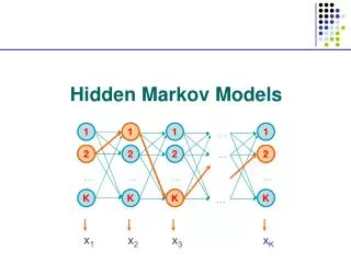
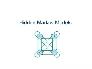
12. Hidden Markov Model (HMM) Delete/skip Insert Match END START M O R N I N G Originally used in speech recognition (Rabiner, 1986) • Proposed for DNA modeling (Churchill, 1989) • Applied to modeling proteins (Haussler et al, 1992) • Multiple sequence alignment • Identification of related family members (“homologs”)

13. Aligning sequences to an HMM to construct an MSA Note: how to read a UCSC a2m-formatted MSA (in-class) http://www.cse.ucsc.edu/research/compbio/ismb99.handouts/KK185FP.html

14. Generating a multiple alignment by aligning sequences to an HMM >Seq6 MIVSTSG >Seq7 MVVTTG >Seq8 SP >Seq9 PP Seq6 M I V S T S G Seq7 M V V - T T G Seq8 - - - - - S P Seq9 - - - - - P P

15. Estimating HMM parameters http://www.cse.ucsc.edu/research/compbio/ismb99.handouts/KK185FP.html

16. http://www.cse.ucsc.edu/research/compbio/ismb99.handouts/KK185FP.htmlhttp://www.cse.ucsc.edu/research/compbio/ismb99.handouts/KK185FP.html

17. Viterbi and Baum-Welch algorithms http://www.cse.ucsc.edu/research/compbio/ismb99.handouts/KK185FP.html

18. Simulated annealing and other methods for handling local optima http://www.cse.ucsc.edu/research/compbio/ismb99.handouts/KK185FP.html

19. Sequence weighting http://www.cse.ucsc.edu/research/compbio/ismb99.handouts/KK185FP.html

20. Henikoff weighting http://www.cse.ucsc.edu/research/compbio/ismb99.handouts/KK185FP.html

21. Henikoff weighting Weight of a character in the MSA = 1/m*k m = #unique amino acids seen k = # times a particular amino acid is seen Weight of a sequence is the average of the weights in all positions, normalized to sum to 1. http://www.cse.ucsc.edu/research/compbio/ismb99.handouts/KK185FP.html

22. Overfitting and regularization http://www.cse.ucsc.edu/research/compbio/ismb99.handouts/KK185FP.html

23. Using pseudocounts http://www.cse.ucsc.edu/research/compbio/ismb99.handouts/KK185FP.html

24. Dirichlet mixture densities http://www.cse.ucsc.edu/research/compbio/ismb99.handouts/KK185FP.html

25. Including prior information in profile or HMM construction The use of Dirichlet mixture densities

26. D S I F M K D S V F M K D T I W M K D T I W M K D T V W M K Profile or HMM parameter estimation using small training sets What other amino acids might be seen at this position among homologs? What are their probabilities? .

27. D S I F M K D S V F M K D T I W M K D T I W L K D T L W L R The context is critical when estimating amino acid distributions This position may be critical for function or structure, and may not allow substitutions .

28. Dirichlet Mixture Prior “Blocks9” Parameters estimated using Expectation Maximization (EM) algorithm. Training data: 86,000 columns from BLOCKS alignment database.

29. ˆ pi = the estimated probability of amino acid ‘i’ n = (n1,…,n20) = the count vector summarizing the observed amino acids at a position. αj = (αj,1 ,…, αj,20 ) = the parameters of component j of the Dirichlet mixture Θ. Combining Prior Knowledge with Observations using Dirichlet Mixture Densities Dirichlet Mixtures: A Method for Improved Detection of Weak but Significant Protein Sequence Homology. Sjolander, Karplus, Brown, Hughey, Krogh, Mian and Haussler. CABIOS (1996)

33. http://www.cse.ucsc.edu/research/compbio/ismb99.handouts/KK185FP.htmlhttp://www.cse.ucsc.edu/research/compbio/ismb99.handouts/KK185FP.html

34. Log-odds ratio http://www.cse.ucsc.edu/research/compbio/ismb99.handouts/KK185FP.html

35. Seq1 M V V S - - P Seq2 M V V S T G P Seq3 M V V S S G P Seq4 M V L S S P P Seq5 M - L S G P P HMM construction using an initial multiple sequence alignment Delete/skip Insert Match

36. In searching for family members, all features must be assumed to be equally informative.

37. Without knowing which features are more important, would we recognize this relative?

38. Gathering family members allows us to identify conserved attributes and create a profile Conserved: stripes, cat. Variable: coat color, size.

39. Profile generalization allows us to identify sometruly remote relatives

40. Conflict • For effective remote homolog detection, a profile or HMM needs information from divergent family members • Without this context, we cannot differentiate critical from variable positions • HMMs constructed with such data provide a coarse classification • But, the more variability we introduce in training data, the greater the potential noiseat some positions D S LF MK I D S IF MK V D T IW MK M D T IW MK L D T VW MK F D T FR DK I D T FR DK V

41. Divergence across the family; conservation within subfamilies Average BLOSUM62 Score Position

42. Subfamily HMM Construction

43. 3.5.2.2 Dihydropyrimidinase 3.5.4.1 Cytosine deaminase 3.5.2.3 Dihydroorotase 3.5.1.5 Urease Subfamily Assessing classification accuracy 7TM GPCR ABC Transporter Amidohydrolase ATPase Family

44. Subfamily HMMs (SHMMs) Discovering and Modeling Functional Subtypes

45. How to build Subfamily HMMs (SHMMs) D S LF MK I D S IF MK V D T IW MK M D T IW MK L D T VW MK F D T FR KK I D T FR KK V Share statistics between subfamilies where there is evidence of a common distribution. 1 2 3 4 5 6 7 Keep statistics separate at positions where there is evidence of divergent structure. 3 4 5 1 2 6 7 Improved specificity, sensitivity, alignment accuracy

46. Step 1: Form Dirichlet Mixture Posterior At each position, for each subfamily, construct a Dirichlet mixture posterior, by combining the Dirichlet mixture prior with the amino acids aligned at that position by that subfamily. (Weighted) subfamily counts Mixture coefficient Component Parameters (Weighted) subfamily counts of amino acid i

47. Step 2: Calculate family contribution Other subfamilies contribute, proportional to the probability of the amino acids they aligned at that position, given the revised Dirichlet mixture density. D S LF MK I D S IF MK V D T IW MK M D T IW MK L D T VW MK F D T FR KK I D T FR KK V (Weighted) counts from subfamily s΄ (Formula for computing Prob (n | Θ ) are in Sjolander et al, 1996)

48. Step 3: Compute pseudocounts Add the family contribution to the observed (weighted) counts, to obtain the pseudocounts ti of amino acid i: (Weighted) subfamily counts for subfamily s family contribution

49. Step 4: Compute amino acid probabilities Normally, we compute amino acid probabilities by combining a Dirichlet mixture prior with observed counts as follows:

50. SHMM Remote Homolog Detection • 515 PFAM Full MSAs, each corresponding to a unique SCOP Fold. • Family HMMs constructed using UCSC SAM w0.5 software. • Subfamily HMMs constructed using BETE. • Each sequence in PDB90 assigned a family score and a subfamily score (best-of-SHMMs). • E-values computed by fitting these scores to an extreme value distribution Brown D, Krishnamurthy N, Dale J, Christopher W, and Sjölander K, "Subfamily HMMs in Functional Genomics", Proceedings of the Pacific Symposium on Biocomputing, 2005