Download
1 / 12
120 likes | 222 Vues
Section 3 # 1. 3. Vertical Data LECTURE 1. In Data Processing, you run up against two curses immediately. Curse of cardinality: solutions don’t scale well with respect to record volume . "files are too deep!"

E N D
Section 3 # 1 3. Vertical Data LECTURE 1 • In Data Processing, you run up against two curses immediately. • Curse of cardinality: solutions don’t scale well with respect to record volume. • "files are too deep!" • Curse of dimensionality:solutions don’t scale with respect to attribute dimension. • "files are too wide!" • The curse of cardinality is a problem in both the horizontal and vertical data worlds! • In the horizontal data world it was disguised as “curse of slow joins”. • In the horizontal world we decompose relations to get good design (e.g., 3rd normal form), but then we pay for that by requiring many slow joins to get the answers we need.
Section 3 # 2 Techniques to address these curses. Horizontal Processing of Vertical Dataor HPVD, instead of the ubiquitous Vertical Processing of Horizontal (record orientated) Data or VPHD. Parallelizing the processing engine. • Parallelize the software engine on clusters of computers. • Parallelize the greyware engine on clusters of people (i.e., enable visualization and use the web...). Again, we need better techniques for data analysis, querying and mining because of: Parkinson’s Law: Data volume expands to fill available data storage. Moore’s law: Available storage doubles every 9 months!
Grasshopper caused significant economic loss each year. TIFF image Yield Map Early infestation prediction is key to damage control. Section 3 # 3 A few HPVD successes: 1. Precision Agriculture Yield prediction: Using Remotely Sensed Imagery (RSI) consists of an aerial photograph (RGB TIFF image taken ~July) and a synchronized crop yield map taken at harvest; thus, 4 feature attributes (B,G,R,Y) and ~100,000 pixels. Producer are able to analyze the color intensity patterns from aerial and satellite photos taken in mid season to predict yield (find associations between electromagnetic reflection and yeild). E.g., ”hi_green&low_red hi_yield”. That is very intuitive. A stronger association, “hi_NIR & low_redhi_yield”, found through HPVD data mining), allows producers to take and query mid-season aerial photographs for low_NIR & high_red grid cells, and where low yeild is anticipated, apply (top dress) additional nitrogen. Can producers use Landsat images of China of predict wheat prices before planting? 2. Infestation Detection (e.g., Grasshopper Infestation Prediction - again involving RSI) Pixel classification on remotely sensed imagery holds much promise to achieve early detection. Pixel classification (signaturing) has many, many applications: pest detection, Flood monitoring, fire detection, wetlands monitoring …
Section 3 # 4 3. Sensor Network Data HPVD • Micro and Nano scale sensor blocks are being developed for sensing • Biological agents • Chemical agents • Motion detection • coatings deterioration • RF-tagging of inventory (RFID tags for Supply Chain Mgmt) • Structural materials fatigue • There will be trillions++ of individual sensors creating mountains of data which can be data mined using HPVD (maybe it shouldn't be called a success yet?).
Situation space ================================== \ CARRIER / Section 3 # 5 4. A Sensor Network Application: CubE for Active Situation Replication (CEASR) Nano-sensors dropped into the Situation space Wherever threshold level is sensed (chem, bio, thermal...) a ping is registered in a compressed structure (P-tree – detailed definition coming up) for that location. Using Alien Technology’s Fluidic Self-assembly (FSA) technology, clear plexiglass laminates are joined into a cube, with a embedded nano-LED at each voxel. .:.:.:.:..::….:. : …:…:: ..: . . :: :.:…: :..:..::. .:: ..:.::.. .:.:.:.:..::….:. : …:…:: ..: . . :: :.:…: :..:..::. .:: ..:.::.. .:.:.:.:..::….:. : …:…:: ..: . . :: :.:…: :..:..::. .:: ..:.::.. The single compressed structure (P-tree) containing all the information is transmitted to the cube, where the pattern is reconstructed (uncompress, display). Each energized nano-sensor transmits a ping (location is triangulated from the ping). These locations are then translated to 3-dimensional coordinates at the display. The corresponding voxel on the display lights up. This is the expendable, one-time, cheap sensor version. A more sophisticated CEASR device could sense and transmit the intensity levels, lighting up the display voxel with the same intensity. Soldier sees replica of sensed situation prior to entering space
Section 3 # 6 3. Anthropology ApplicationDigital Archive Network for Anthropology (DANA)(analyze, query and mine arthropological artifacts (shape, color, discovery location,…)
visualization Pattern Evaluation and Assay Data Mining Classification Clustering Rule Mining Loop backs Task-relevant Data Data Warehouse: cleaned, integrated, read-only, periodic, historical database Selection Feature extraction, tuple selection Raw data must be cleaned of: missing items, outliers, noise, errors Smart files Section 3 # 7 What has spawned these successes?(i.e., What is Data Mining?) Queryingis asking specific questions for specific answers Data Mining is finding the patterns that exist in data (going into MOUNTAINS of raw data for the information gems hidden in that mountain of data.)
Fractals, … Standard querying Searching and Aggregating Data Prospecting Machine Learning Data Mining Association Rule Mining OLAP (rollup, drilldown, slice/dice.. Supervised Learning – classification regression SQL SELECT FROM WHERE Complex queries (nested, EXISTS..) FUZZY query, Search engines, BLAST searches Unsupervised Learning - clustering Walmart vs.KMart Section 3 # 8 Data Mining versus Querying There is a whole spectrum of techniques to get information from data: Even on the Query end, much work is yet to be done(D. DeWitt, ACM SIGMOD Record’02). On the Data Mining end, the surface has barely beenscratched. But even those scratches have had a great impact. For example, one of the early scatchers became the biggest corporation in the world. A Non-scratcher had to file for bankruptcy protection. HPVD Approach:Vertical, compressed data structures, Predicate-trees or Peano-trees (Ptrees in either case)1 processed horizontally (Most DBMSs processhorizontal data vertically) • Ptrees are data-mining-ready, compressed data structures, which attempt to address the curses of cardinality and curse of dimensionality. 1 Ptree Technology is patented by North Dakota State University
Predicate trees (Ptrees): vertically project each attribute, R[A1] R[A2] R[A3] R[A4] 010 111 110 001 011 111 110 000 010 110 101 001 010 111 101 111 011 010 001 100 010 010 001 101 111 000 001 100 111 000 001 100 010 111 110 001 011 111 110 000 010 110 101 001 010 111 101 111 011 010 001 100 010 010 001 101 111 000 001 100 111 000 001 100 for Horizontally structured records Scan vertically = pure1? true=1 pure1? false=0 R11 R12 R13 R21 R22 R23 R31 R32 R33 R41 R42 R43 0 1 0 1 1 1 1 1 0 0 0 1 0 1 1 1 1 1 1 1 0 0 0 0 0 1 0 1 1 0 1 0 1 0 0 1 0 1 0 1 1 1 1 0 1 1 1 1 0 1 1 0 1 0 0 0 1 1 0 0 0 1 0 0 1 0 0 0 1 1 0 1 1 1 1 0 0 0 0 0 1 1 0 0 1 1 1 0 0 0 0 0 1 1 0 0 pure1? false=0 pure1? false=0 pure1? false=0 0 0 0 1 0 01 0 1 0 1 0 1 1. Whole is pure1? false 0 P11 P12 P13 P21 P22 P23 P31 P32 P33 P41 P42 P43 2. Left half pure1? false 0 P11 0 0 0 0 1 01 3. Right half pure1? false 0 0 0 0 0 1 0 0 10 01 0 0 0 1 0 0 0 0 0 0 0 1 01 10 0 0 0 0 1 0 0 0 0 1 0 0 0 0 1 0 0 0 0 0 0 0 0 0 0 1 0 0 ^ ^ ^ ^ ^ ^ ^ 0 0 1 0 1 4. Left half of rt half? false0 0 0 1 0 1 01 5. Rt half of right half? true1 0 1 0 Section 3 # 9 1-Dimensional Ptrees then vertically project each bit position of each attribute, Given a table structured into horizontal records. (which are traditionally processed vertically - VPHD ) then compress each bit slice into a basic 1D Ptree. e.g., compression of R11 into P11 goes as follows: =2 VPHD to find the number of occurences of 7 0 1 4 HPVD to find the number of occurences of 7 0 1 4? R(A1 A2 A3 A4) Base 10 Base 2 2 7 6 1 6 7 6 0 3 7 5 1 2 7 5 7 3 2 1 4 2 2 1 5 7 0 1 4 7 0 1 4 R11 0 0 0 0 0 0 1 1 Top-down construction of the 1-dimensional Ptree of R11, denoted, P11: Record the truth of the universal predicate pure 1 in a tree recursively on halves (1/21 subsets), until purity is achieved. P11 To find the number of occurences of 7 0 1 4, AND these basic Ptrees (next slide) But it is pure (pure0) so this branch ends
R[A1] R[A2] R[A3] R[A4] 010 111 110 001 011 111 110 000 010 110 101 001 010 111 101 111 101 010 001 100 010 010 001 101 111 000 001 100 111 000 001 100 010 111 110 001 011 111 110 000 010 110 101 001 010 111 101 111 101 010 001 100 010 010 001 101 111 000 001 100 111 000 001 100 = R11 R12 R13 R21 R22 R23 R31 R32 R33 R41 R42 R43 0 1 0 1 1 1 1 1 0 0 0 1 0 1 1 1 1 1 1 1 0 0 0 0 0 1 0 1 1 0 1 0 1 0 0 1 0 1 0 1 1 1 1 0 1 1 1 1 1 0 1 0 1 0 0 0 1 1 0 0 0 1 0 0 1 0 0 0 1 1 0 1 1 1 1 0 0 0 0 0 1 1 0 0 1 1 1 0 0 0 0 0 1 1 0 0 0 1 0 1 0 0 0 0 1 0 01 0 1 0 0 1 01 This 0 makes entire left branch 0 7 0 1 4 These 0s make this node 0 P11 P12 P13 P21 P22 P23 P31 P32 P33 P41 P42 P43 These 1s and these 0s(which when complemented are 1's)make this node1 0 0 0 0 1 01 0 0 0 0 1 0 0 10 01 0 0 0 1 0 0 0 0 0 0 0 1 01 10 0 0 0 0 1 10 0 1 0 ^ ^ ^ ^ ^ ^ ^ ^ ^ 0 0 1 0 1 0 0 1 0 1 01 0 1 0 Section 3 # 10 R(A1 A2 A3 A4) 2 7 6 1 3 7 6 0 2 7 5 1 2 7 5 7 5 2 1 4 2 2 1 5 7 0 1 4 7 0 1 4 # change To count occurrences of 7,0,1,4 use 111000001100: 0 P11^P12^P13^P’21^P’22^P’23^P’31^P’32^P33^P41^P’42^P’43 = 0 0 01 The 21-level has the only 1-bit so 1-count = 1*21 = 2 ^
R11 0 0 0 0 1 0 1 1 Top-down construction of basic P-trees is best for understanding, bottom-up is much faster (once across). 0 0 0 0 1 0 0 0 0 0 0 1 1 1 Section 3 # 11 Bottom-up construction of 1-Dim, P11, is done using in-order tree traversal, collapsing of pure siblings as we go: P11 R11 R12 R13 R21 R22 R23 R31 R32 R33 R41 R42 R43 0 1 0 1 1 1 1 1 0 0 0 1 0 1 1 1 1 1 1 1 0 0 0 0 0 1 0 1 1 0 1 0 1 0 0 1 0 1 0 1 1 1 1 0 1 1 1 1 1 0 1 0 1 0 0 0 1 1 0 0 0 1 0 0 1 0 0 0 1 1 0 1 1 1 1 0 0 0 0 0 1 1 0 0 1 1 1 0 0 0 0 0 1 1 0 0 0 Siblings are pure0 so callapse!
Section 3 Please proceed to 03_Vertical_data_LECTURE2