SIO ‘Spray’ Gliders for ASAP

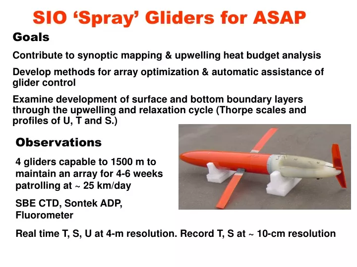
1. SIO ‘Spray’ Gliders for ASAP Goals Contribute to synoptic mapping & upwelling heat budget analysis Develop methods for array optimization & automatic assistance of glider control Examine development of surface and bottom boundary layers through the upwelling and relaxation cycle (Thorpe scales and profiles of U, T and S.) Observations 4 gliders capable to 1500 m to maintain an array for 4-6 weeks patrolling at ~ 25 km/day SBE CTD, Sontek ADP, Fluorometer Real time T, S, U at 4-m resolution. Record T, S at ~ 10-cm resolution

2. Maintaining Glider Arrays • The error from objective mapping provides a metric for optimizing sampling arrays. • Fratantoni’s rule: A good array should yield data that can be analyzed without model assimilation (WOMA). • Direct minimization of mapping error leads to arrays that are not very useful WOMA. • 4. A hybrid approach – specify general structure of array to make data useable WOMA and adjust the parameters of these structures to optimize mapping skill.

3. Direct Optimization A glider is imagined to produce a sample every dt while traveling at speed U After each dt the glider is allowed to adopt a new heading Each track is given the score equal to the time integral of the mapping error over some specified rectangular region The mapping error is based on a homogeneous stationary signal covariance of the form C = A exp [-(x1-x2)2/L2-(y1-y2)2/L2-(t1-t2)2/T2 which it makes it feasible to compute the area-average square error analytically.

4. What are the Scales L and T? Even combined WHOI & SIO AOSN-II glider data does not define the full anisotropic and inhomogeneous covariance. Appropriate “mean” temperature is A(t) + B(t) x Doffshore

5. Evidence for anisotropy and offshore dependence of scales is weak Scales of Temperature Depth Half variance in noise Cross-Shelf slightly longer than alongshore

6. Isotropic Correlation of Temperature Depth Weak dependence on offshore distance 0.5 Correlation L ~ 15 km T ~ 2 days

7. Direct Optimization Results Unless constrained by the boundaries of the area of interest or by a nearby sample, “optimal” trajectories tend to be aimless wandering around an area of one correlation length on a side. These array paths are not useful WOMA although they score well in area average mapping error.

8. Example of Direct Optimization

9. (Naomi’s) Hybrid Approach Design generalized arrays of glider tracks that would allow interpretation WOMA. Then use objective mapping skill to optimize parameters of the generalized array. Modest expansion of the search for optimal a, b and c might provide assistance in dealing with unplanned factors like failures or the need to re-power some gliders b a c

10. 5 gliders 100 km x 30 km One vehicle per racetrack, all moving in the same directions and at the same position of their own racetrack.

11. 5 gliders 100 km x 80 km One vehicle per racetrack, all moving in the same directions and at the same position of their own racetrack.