Download
1 / 24
370 likes | 992 Vues
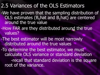
Properties of OLS. How Reliable is OLS?. Learning Objectives. Review of the idea that the OLS estimator is a random variable How do we judge the quality of an estimator? Show that OLS is unbiased Show that OLS is Consistent Show that OLS is efficient The Gauss-Markov Theorem.

E N D
Properties of OLS How Reliable is OLS?
Learning Objectives • Review of the idea that the OLS estimator is a random variable • How do we judge the quality of an estimator? • Show that OLS is unbiased • Show that OLS is Consistent • Show that OLS is efficient • The Gauss-Markov Theorem
1. OLS is a Random Variable • An Estimator is any formula/algorithm that produces an estimate of the “truth” • An estimator is a function of the sample data e.g. OLS • Others: “Draw a line” • For individual consumption function its not so obvious • Implications for accuracy of the estimates • So how do we choose between different estimators? • What are the criteria • What is so special about OLS? • What does it take for OLS to go wrong?
Recall the Definition of OLS • Review of where OLS comes from. • Think of fitting a line to the data. This will never pass through every point • Every choice of b0 and b1 will generate a new set of ui • OLS chooses b0 and b1 to min sum of squared ui • “Best fit” • R2 • so what?
OLS Formulae • The key issue is that both are functions of the data so the precise value of each estimate will depend on the particular data points included in the sample • This observation is basis of all statistical inference and all judgments regarding the quality of estimates.
Distribution of Estimator • Estimator is a random variable because sample is random • “Sampling error” or “Sampling distribution of the estimator” • To see the impact of the sampling on estimates, try different samples (see histograms over) • Key point: even if we have the correct model we could get an answer that is way off just because we are unlucky in the sample. • How do we know if we have been unlucky? How can we minimise the chances of bad luck? • This is basically how we assess the quality of one estimation procedure compared to another
Comparing MAD and OLS • Both estimators are random variables • The OLS estimator has lower variance than the MAD distribution • Both are centred around the true value of beta (0.75)
How Judge an Estimator? • Comparing estimators amounts to comparing distributions • Estimators are judged on three criteria • Unbiased • Consistent • Efficient • These criteria are all different takes on the question of: what is the probability that I will get a seriously wrong answer from my regression? • OLS is the Best Linear Unbiased Estimator (BLUE) • Gauss-Markov Theorem • This is why it is used
2. Bias • Sampling distribution of the estimator is centered around the true value • E(bOLS)=b • Implication: With repeated attempts OLS will give correct answer on average • Does not imply that it will give the correct answer in any given regression • Consider the stylized distribution of two estimators below • The OLS estimator is centered around the true value. The alternative is not • Is OLS better? • Suppose your criteria were the avoidance of really small answers? • Unbiasedness hinges on the model being correctly specified i.e. correct variables • Omitted relevant variables • It doesn’t require a large number of observations: “small sample” • Both MAD and OLS are unbiased
OLS is centered around the true value but has a relatively high probability of returning a value that is low
3. Consistency • Consistency is a large sample property i.e. asymptotic property • As N , the distribution of the estimator collapse to the true value • The distribution gets narrower • This is more useful than unbiasedness because it implies that the probability of getting any wrong answer falls as sample size increases • Formalises the common intuition that more data is better • “Law of Large Numbers” • Note an estimator could be biased but still consistent e.g. 2SLS • Consistency requires a correctly specified model
Same estimator, Larger sample As sample size increases we get closer to truth e.g. prob of error falls
4. Efficiency • An efficient estimator has minimum variance of all possible alternatives • Squashed distribution • Looks similar to consistency but is small sample property • Compares different estimators applied to the same sample • OLS is efficient i.e. “best” • Reason why it is used where possible • GLS, IV, WLS, 2SLS are inefficient • OLS is more efficient in our example than MAD
Same sample size, different estimator Prob of error is lower for efficient estimator at any sample size
5. Gauss-Markov Theorem • A formal statement of what we have just discussed • Mathematical specification is required in order to do hypothesis tests • Standard model • Observation = systematic component + random error: • yi = 1 +2 xi + ui • Sample regression line estimated using OLS estimators: • yi = b1 + b2 xi + ei
Assumptions • Linear Model ui = yi - 1- 2xi • Error terms have mean = 0 • E(ui|x)=0 => E(y|x) = 1 + 2xi • Error terms have constant variance (independent of x) • Var(ui|x) = 2=Var(yi|x) (homoscedastic errors) • Cov(ui, ui )= Cov(yi, yi )= 0. (no autocorrelation) • X is not a constant and is fixed in repeated samples. • Additional assumption: • ui~N(0, 2) => yi~N(1- 2xi, 2)
Summary BLUE • Best Linear Unbiased Estimator • Linear: Linear function of the data • Unbiased: Expected Value of the estimator equals true value • Doesn’t mean always get the correct answer • Algebraic proof in book • Unbiasedness property hinges on the model being correctly specified i.e. E(xi ui)=0
Some Comments On BLUE • Aka Gauss-Markov Theorem: • First 5 assumptions above must hold • OLS estimators are the “best” among all linear and unbiased estimators because • they are efficient: i.e. they have smallest variance among all other linear and unbiased estimators • G-M result does not depend on normality of dependent variable • Normality comes in when we do hypothesis tests • G-M refers to the estimators b1, b2, not to actual values of b1, b2 calculated from a particular sample • G-M applies only to linear and unbiased estimators, there are other types of estimators which we can use and these may be better in which case disregard G-M • a biased estimator may be more efficient than an unbiased one which fulfills G-M.
Conclusions • OLS estimator is a random variable: • its precise value varies with the particular sample used • OLS is unbiased: • the distribution is centred on the truth • OLS is Consistent: • Probability of large error falls with sample size
OLS is efficient: • Probability of large error is smallest of all possible estimators • The Gauss-Markov Theorem: • formal statement that 3-5 hold when certain assumptions are true
What’s Missing? • What happens to OLS when the assumptions of the GM theorem are violated • There will be some other estimator that will be better • We will look at 4 violations: • Omitted variable bias • Multicolinearity • Heteroscedastcity • Autocorrelation