Download

1 / 72
720 likes | 854 Vues
Biostat 200 Lecture 2. Today. Discussion/demo of data cleaning Probability Definitions Examples of use in diagnostic tests. Data cleaning. Data cleaning is always necessary with a new data set Assume your data set has errors and your job is to find them

E N D
Today • Discussion/demo of data cleaning • Probability • Definitions • Examples of use in diagnostic tests
Data cleaning • Data cleaning is always necessary with a new data set • Assume your data set has errors and your job is to find them • Use tables and summary statistics and graphs to identify problems, outliers and anomalies • Outliers • Extreme values, numerically distant from the bulk of the data • We do NOT automatically remove outliers !!! • Carefully document all decisions to drop or change values • Always keep a copy of the original data
Pocket change data • I read in the data use "H:\Work files\Teaching\Biostat 200-- 2012\pocket change.dta", clear • and ran summarize and got: . summ var1 Variable | Obs Mean Std. Dev. Min Max -------------+-------------------------------------------------------- var1 | 0 • This showed that there was no data…
Pocket change data • To check this I could have run codebook codebook var1 ------------------------------------------------------------------------------------------------------- var1 (unlabeled) ------------------------------------------------------------------------------------------------------- type: string (str8) unique values: 39 missing "": 4/51 examples: "0" "133" "30" "54" warning: variable has embedded blanks
Pocket change data • For var2 .codebook var2 ------------------------------------------------------------------------------------------------------- var2 (unlabeled) ------------------------------------------------------------------------------------------------------- type: numeric (byte) range: [1,2] units: 1 unique values: 2 missing .: 0/51 tabulation: Freq. Value 12 1 39 2 • Codebook without any names after will run for all the variables in your data set
Pocket change data • I could also have run “describe” . describe Contains data from H:\Work files\Teaching\Biostat 200-- 2012\pocket change.dta obs: 51 vars: 2 18 Sep 2012 16:33 size: 663 (99.9% of memory free) ---------------------------------------------------------------------------------------------------------------------------- storage display value variable name type format label variable label ---------------------------------------------------------------------------------------------------------------------------- var1 str8 %9s var2 byte %8.0g -----------------------------------------------------
Pocket change data • To see the values of var1: tab var1 • To recode the data I ran (see file make_pocketchange.do): .generate cents=var1 .replace cents= "92" if var1=="92 cents" .tab cents, missing .destringcents, replace force .tab cents .drop var1 .hist cents, fcolor(blue) lcolor(black) width(25) percent title("Distribution of change in Biostat 200") New variable name that I made up
Pocket change data • What about unexpected values? Are these values possible? Are they extreme? 1.06 cents? 7.1 cents? 402 cents?
Outliers – what do we do? • First consider if the value is physically possible • 402 cents is possible, the others are not • Look at the other variables for clues. In this data set we don’t have anything else to look at (except sex) – but we will see in other data that sometimes this other variables are useful • Document all changes to data • Always retain a copy of the original data set
Outliers – what do we do? • What about outliers that seem reasonable? • Remember outliers are distant from the rest of the data, that doesn’t mean they are wrong • Keep them, but • Be aware that they may have large influence on some analyses • Think about more robust analyses (analyses not so sensitive to extreme values) • E.g. which measures of central tendency might you use?
Pocket change data • Here we decided to delete values (1.06 and 7.1) that aren’t possible but keep those that are (402) ** drop these 2 observations due to invalid values ** drop if cents==1.06 | cents==7.1 • These commands written in .do file • Use comments bracketed by ***s to remind why these values are dropped • Save data to a new file (so that original data are preserved) save “pocket change_edited_2012_0923.dta"
Outliers • Sometimes other variables help determine whether or not to keep outliers • Class data: Weight<100 lbs list htfthtinchhtcmwtlbswtkg sex age if wtlbs<100 +-------------------------------------------------+ | htfthtinchhtcmwtlbswtkg sex age | |-------------------------------------------------| 2. | 6 0 181 38 80 0 36 | 49. | 5 0 90 . 1 70 | 105. | 5 3 159 29 63 1 34 | 106. | 5 8 170 35 74 0 37 | 107. | 5 3 159 33 63 1 34 | |-------------------------------------------------| 108. | 5 7 172 36 76 0 37 | 416. | 5 0 80 . 1 20 | 421. | 4 11 80 . 1 28 | +-------------------------------------------------+
An ounce of prevention • Make sure numbers are coded as such – do not allow text • Range checks, skip patterns • Most programs (other than excel spreadsheets) have such capabilities • Do double entry if data were not collected electronically • Examine the data as early and as frequently as possible to check for problems
Basic probability • Probability is the foundation of statistical inference • Statistical inference is what is needed to make statements about the characteristics of the population from which a sample was drawn • p-values and confidence intervals tell us how our sample might relate to the population • Many of the entities we use daily are probabilities – e.g. the probability of breast cancer given a patient is BRCA1/2 positive Population Sample
Basic probability • Event • Result of an experiment or observation • Occurs or does not occur • Denoted by uppercase letters e.g. A,B, X • We will apply probability to events • We want to the relative frequency that an event occurs over a large number of identical trials • E.g. • An event may be a disease occurrence or a large laboratory value
Basic probability Frequentist definition of probability • If an experiment is repeated n times under essentially identical conditions, and if the event A occurs m times, then as n increases, • the ratio m/n approaches a fixed number the probability of A • P(A) = m/n
Basic probability • Probability of an event – relative frequency of its occurrence in a large number of trials repeated under the same conditions • E.g. Probability of picking a red ball out of a bag of red and black balls • Always lies between 0 and 1 (inclusive) • Denoted P(A) or P(X)
A A Ā Basic probability Complement of an event, Ā or AC (read Not A or A complement) • E.g. A is the event that a person has Plasmodium falciparum (P.f.) malaria, Ā is the event of no P.f. malaria • P(A)= 1-P(Ā) • Often E for exposed and Ē for not exposed
A A Ā Basic probability UniverseΩ is all the possible outcomes of an event • P(Ω) = P(A) + P(Ā) = 1 Ω
Complement example • Probability that someone has Plasmodium falciparum (P.f.) malaria plus the probability that they do not • P(P.f.+) + P(P.f.-) = 1
Basic probability • The intersection of 2 events is written A ∩ B • The intersection is when both A and B occur • E.g. The event that a person has both malaria and pulmonary tuberculosis • The probability that both occur is written P(A ∩ B) A A ∩ B B
Basic probability • The union of 2 events is written A U B • The union is if either A or B or both occur • E.g. The event that a person has either malaria or tuberculosis or both • P(A U B) = P(A) + P(B) – P(A ∩ B) • The probability of A or B is the sum of their individual probabilities minus the probability of their intersection A A ∩ B B
Basic probability • Two events are mutually exclusive if they cannot occur together • There is no overlap area because both can’t happen together • The intersection is empty • E.g. • Being pregnant and not pregnant • You cannot be both B A
Basic probability • For mutually exclusive events, the probability of A or B occurring is the sum of their individual probabilities • Both A and B cannot occur together so P(A ∩ B) = 0 • P(A U B) = P(A) + P(B) - P(A ∩ B) = P(A) + P(B) B A
Basic probability • If A and B are mutually exclusive, P(A U B) = P(A) + P(B) • This is the additive rule of probability • E.g. Among persons with HCV infection (assuming one infection at a time) P(HCV genotype 1) in the US = .7 P(HCV genotype 2) in the US = .15 P(All other HCV genotypes) = .15 P(HCV genotype 1 or 2) = .7 + .15 = .85
Basic probability • The additive rule of probability can be applied to three or more mutually exclusive events • If none of the events can occur together, then P(A1 U A2 U A3 ) = P(A1) + P(A2) + P(A3) For n events: P(A1 U A2 U … U An ) = P(A1) + P(A2) + … P(An)
Probability summary • Complement: P(A)= 1-P(Ā) • Intersection: Prob A and B = P(A ∩ B) • Union: Prob A or B or both = P(A U B) P(A U B) =P(A) + P(B) – P(A ∩ B) • Mutually exclusive events: P(A ∩ B) = 0 P(A U B) = P(A) + P(B) additive rule
Probability summary • Are A and Ā (i.e. an event and its complement) mutually exclusive? • What is P(A ∩ Ā) ? • What is P(A U Ā) ?
Basic probability example • A = the event that an individual is exposed to high levels of carbon monoxide • B = the event that an individual is exposed to high levels of nitrogen dioxide • What is the event A ∩ B called? What is that in this example? • What is the event A U B called? What is it in this example? • What is the complement of A? • Are A and B mutually exclusive?
Basic probability example • A ∩ B is the intersection of A and B. It is the event that the person is exposed to both gases. • A U B is the union of A and B. It is the event that the person is exposed to one or the other or both. • Ā is the event that the person is not exposed to carbon monoxide. • Are A and B mutually exclusive? Can they both occur? Yes. So they are NOT mutually exclusive.
Conditional probability • The probability that an event B will occur given that event A has occurred • Notation: P(B|A) • Read: the probability of B given A • Example: Probability of a person becoming infected with malaria given that he/she uses a bed net at night • Event A is using a bed net • Event B is becoming infected with P.f. malaria
Conditional probability P(B|A) = P(A ∩ B) / P(A) The probability of B given A is the probability of the intersection (i.e. both events occurring) divided by the probability of A occurring It is the relative size of the probability of the intersection A ∩ B compared to the relative size of the probability of A occurring B A A ∩ B
Conditional probability example P(becoming infected with malaria | use a bed net) = P(B|A) = P(A ∩ B) / P(A) = P( Becoming infected and using a bed net ) / P(using a bed net) Estimated by: proportion of people who become infected with malaria and who use a bed net / proportion of people who use a bed net or number of people who become infected with malaria and who use a bed net / number of people who use a bed net
Conditional probability • Multiplicative rule of probability P(A ∩ B) = P(A) P(B|A) The probability of both A and B occurring is the probability A will occur times the probability that B will occur given that A has occurred. This is a rearrangement of the definition of conditional probability Also: P(A ∩ B) = P(B ∩ A) = P(B) P(A|B)
Probability example 1992 U.S. birth statistics • Because the sample is so large the proportion approaches the probability • Probability that mother’s age was 20-24 = 0.263 • Probability that mother’s age was ≤24 = 0.003 + 0.124 + 0.263 = 0.390 • By what probability rule? • What was the mode for maternal age at delivery?
Probability example 1992 U.S. birth statistics • Given that a mother is under age 30, what is the probability that she is under age 15? P( Mother’s age<15 | Mother’s age<30 ) = P ( Mother’s age<15 and <30 ) / P(Mother’s age <30) = ( 0.003) / ( 0.003 + 0.124 + 0.263 + 0.290 ) = 0.003 / 0.68 = 0.004
Examples of conditional probabilities • Relative risk is the ratio of 2 conditional probabilities RR = P(disease | exposed) / P(disease | not exposed) • Odds ratios also include conditional probabilities OR =P(disease | exposed) / (1- P(disease | exposed)) / P(disease | not exposed) / (1- P(disease | not exposed))
Independence • If the occurrence of B does not depend on A, then by the definition of independence, P(B|A) = P(B) • Example: Probability of becoming infected with P.f. malaria given that you have 2 sisters = probability of becoming infected with P.f. malaria • Then the multiplicative rule P(A ∩ B) = P(A) P(B|A) reduces to P(A ∩ B) = P(A) P(B) • Example: coin tosses – the probability of a heads on the 2nd throw is independent of the outcome on the first throw
Independence Note that independence ≠ mutual exclusivity! • Mutual exclusivity • 2 events cannot both occur • P(A ∩ B) =0 • Independence • 2 events do not depend on each other P(B|A)=P(B) • P(A ∩ B) = P(A) P(B|A) = P(A) P(B)
Law of Total Probability • The law of total probability: P(B) = P(B ∩ A) + P(B ∩ Ā) P(B) = P(B|A)P(A) + P(B|Ā)P(Ā) More generally, if you can divide A into multiple mutually exclusive (non-overlapping) sections (here n=5): P(B) = P(B ∩ A1) + P(B ∩ A2) + … + P(B ∩ An) P(B) = P(B|A1)P(A1) + P(B|A2)P(A2) + … + P(B|An)P(An)
Law of Total Probability • Helpful when you cannot directly calculate a probability • Example: • Suppose you know the TB prevalence in different areas and the population size in those areas, and you want to know the worldwide TB prevalence • P(TB+) = P(TB+| live in lower income country)*P(live in lower income country) + P(TB+| live in upper income country)*P(live in upper income country) • Weighted average of the 2 TB prevalences
Diagnostic tests • Diagnostic tests of disease are rarely perfect • True positives – the test is positive given the person has the disease • The probability of this is P(T+|D+) = Sensitivity • False positives – the test is positive although the person does not have the disease • True negatives – the test is negative given the person does not have the disease • The probability of this is P(T-|D-) = Specificity • False negatives – the test is negative even though the person has the disease
Diagnostic tests • Divide the world into 4 quadrants based on disease and test result • Sensitivity = P(T+|D+) = P(T+∩D+)/P(D+) = TP/(TP+FN) • Specificity = P(T-|D-) = P(T-∩D-)/P(D-) = TN/(FP+TN)
Diagnostic tests • Diagnostic test characteristics (sensitivity and specificity) are based on experiments in which a test is compared to a “gold standard”=“truth”
Diagnostic test validation example • New biological markers of alcohol consumption are being developed. Phosphatidylethanol (PEth) is a metabolite of alcohol that is formed only in the presence of alcohol and lasts 2-3 weeks after moderate drinking. • We examined 77 persons with HIV in Mbarara, Uganda. We followed them for 21 days and did daily breathalyzers and drinking surveys. If the breathalyzer result was ever >0 and/or the participant reported drinking, we considered this any alcohol consumption (“true drink+”). • We drew blood at the end of the 21-days to test for PEth.
Diagnostic test example • Sensitivity = P(PEth Test+ | true drink+) = TP/(TP+FN) = ??? • Specificity = P(PEth Test - | true drink-) = TN /(TN + FP) = ???
Diagnostic tests • Test results are often a continuous value (i.e. an optical density in an ELISA test) • The level of the cutoff for a diagnostic test can be set to • Maximize sensitivity • This might be ideal if a follow up confirmatory test is easy and you want to be sure not to miss any positives • Maximize specificity • This might be necessary if there are grave ramifications of a false positive test • When you change the cut point to maximize sensitivity you decrease specificity and vice-versa