Download
1 / 31
370 likes | 964 Vues
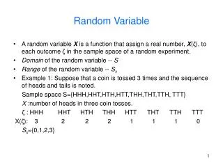
Chapter 6 Normal Random Variable. Chapter 6 Normal Random Variable. 6.1 Introduction 6.2 Continuous Random Variables 6.3 Normal Random Variables 6.4 Probabilities Associated with a Standard Normal Random Variable 6.5 Finding Normal Probabilities: Conversion to the Standard Normal

E N D
Chapter 6 Normal Random Variable 6.1 Introduction 6.2 Continuous Random Variables 6.3 Normal Random Variables 6.4 Probabilities Associated with a Standard Normal Random Variable 6.5 Finding Normal Probabilities: Conversion to the Standard Normal 6.6 Additive Property of Normal Random Variables 6.7 Percentiles of Normal Random Variables
Introduction • In this chapter we introduce and study the normal distribution. • The normal distribution is one of a class of distributions that are called continuous. • The standard normal distribution is a normal distribution having mean 0and variance 1. • The normal distribution was introduced by the French mathematician Abraham De Moivre in 1733.
Continuous Random Variable • A continuous random variable is one whose set of possible values is an interval. • For example, such variables as the time it takes to complete a scientific experiment and the weight of an individual are usually considered to be continuous random variables. • Every continuous random variable X has a curve associated with it. • This curve, formally known as a probability density function, can be used to obtain probabilities associated with the random variable. • Consider any two points a and b, where a is less than b. • The probability that X assumes a value that lies between a and b is equal to the area under the curve between a and b. P{a ≤ X ≤ b} = area under curve between a and b • Figure 6.1 presents a probability density function. • The total area under the density curve must equal 1. P{a ≤ X ≤ b} = P{a < X < b}
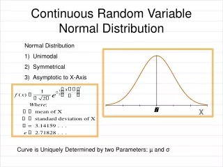
Normal Random Variables • The probability density function of a normal random variable Xis determined by two parameters: • the expected value (μ) and • the standard deviation (σ) of X. • The normal probability density function is a bell-shaped density curve that is symmetric about the value μ. • Its variability is measured by σ. • The larger σ is, the more variability there is in this curve.
Normal Random Variables • The probability density function of a normal random variable X is symmetric about its expected value μ. P{X < μ} = P{X > μ} = ½ • Not all bell-shaped symmetric density curves are normal. • The height of the normal density curve above point xon the abscissa (橫座標)is • A standard normal random variable is a normal random variable having meanvalue 0 and standard deviation 1, and its density curve is called the standardnormal curve. • The letter Z is used to represent a standard normal random variable.
Example 6.1 • Test scores on the Scholastic Aptitude Test (SAT) verbal portion (口說部份) are normally distributed with a mean score of 504. • If the standard deviation of a score is 84, then we can conclude that • Approximately 68 percent of all scoresare between 504 − 84 = 420and 504 + 84 = 588. • Approximately 95 percent of themare between 504 − 168 = 336 and 504 + 168 = 672. • Approximately 99.7 percent are between 252 and 756.
Exercise (p. 269, 2; 3, 4) • The heights of a certain population of males are normally distributed with mean 69 inches and standard deviation 6.5 inches. Approximate the proportion of this population whose height is less than 82 inches. • Let Z refer to a standard normal random variable. Draw a picture in each case to justify your answer. (1) P{−2 < Z < 2} is approximately (a) 0.68 (b) 0.95 (c) 0.975 (d) 0.50 (2) P{Z > −1} is approximately (a) 0.50 (b) 0.95 (c) 0.84 (d) 0.16
Probabilities Associated with a Standard Normal Random Variable • Let Z be a standard normal random variable. • For each nonegative value of x, Table 6.1 specifies the probability that Z is less than x. (P{Z < x})
Probabilities of Random Variable Z • For each nonnegative value of x, Table 6.1 specifies the probability that Z is less than x. • For instance, P{Z < 1.22} = 0.8888 • We can also use Table 6.1 to determine the probability that Zis greater than x. P{Z ≤ 2} + P{Z > 2} = 1 P{Z > 2} = 1 − P{Z ≤ 2} = 1 − 0.9772 = 0.0228
Example 6.2 • Find (a) P{Z < 1.5} (b) P{Z ≥ 0.8} • Solution (a) From Table 6.1, P{Z < 1.5} = 0.9332 (b) From Table 6.1, P{Z < 0.8} = 0.7881 P{Z ≥ 0.8} = 1 − 0.7881 = 0.2119
Example 6.3 • Find (a) P{1 < Z < 2} (b) P{−1.5 < Z < 2.5} • Solution (a )P{1 < Z < 2} = P{Z < 2} − P{Z < 1} = 0.9772 − 0.8413= 0.1359 (b) P{−1.5 < Z < 2.5} = P{Z < 2.5} − P{Z < −1.5} = P{Z < 2.5} − P{Z > 1.5} = 0.9938 − (1 − 0.9332)= 0.9270
Example 6.4 • Find P{|Z|> 1.8} • Solution (a )P{ |Z| >1.8} = 2P{Z >1.8 } = 2(1 − 0.9641) = 0.0718 • In general, for any value of x and any positive value of a P{Z < −x} = P{Z > x} = 1 − P{Z < x} P{|Z| > a} = P{Z > a} + P{Z < −a} = 2P{Z> a} P{−a < Z < a} = 2P{Z < a} − 1
Exercise (p. 276, 5; p.277, 6, 7) • Argue, using either pictures or equations, that for any positive value of a, P{−a < Z < a}=2P{Z < a}−1 • Find (a) P{−1< Z <1} (b) P{|Z| < 1.4} • Find the value of x, to two decimal places, for which (a) P{Z > x}= 0.05 (e) P{Z < x}= 0.66 (g) P{|Z| < x}= 0.75
Finding Normal Probabilities: Conversion to the Standard Normal • Let Xbe a normal random variable with mean μ and standard deviation σ. • We can determine probabilities concerning Xby using the standard normal distribution Z Z = (X − μ) /σ • Suppose we want to compute P{X < a}. Since X < a is equivalent to the statement where Z is a standard normal random variable.
Example 6.6 • IQ examination scores for sixth-graders are normally distributed with mean value 100and standard deviation 14.2. (a)What is the probability a randomly chosen sixth-grader has a score greater than 130? (b)What is the probability a randomly chosen sixth-grader has a score between 90 and 115? • Solution • Let Xdenote the score of a randomly chosen student. the standard normal distribution Zcan be calculated (a) (b)
Example 6.7 • LetX be normal with mean μ and standard deviation σ. Find (a) P{|X − μ| > σ} (b) P{|X − μ| >2σ} (c)P{|X − μ| > 3σ} • Solution Z = (X − μ) /σ
Additive Property of Normal Random Variables • Notice that
Example 6.8 • Suppose the amount of time a light bulb works before burning out is a normal random variable with mean 400 hours and standard deviation 40 hours. • If an individual purchases two such bulbs, one of which will be used as a spare to replace the other when it burns out, what is the probability that the total life of the bulbs will exceed 750 hours? • Solution • Let X is the life of the bulb used first and Y is the life of the other bulb. • The mean and the deviation of X+Y are 800 and respectively. • Therefore, there is an 81 percent chance that the total life of the two bulbs exceeds 750 hours.
Example 6.9 • Data from the U.S. Department of Agriculture (農業部) indicate that the annual amount of apples eaten by a randomly chosen woman is normally distributed with a mean of 19.9 pounds and a standard deviation of 3.2 pounds, whereas the amount eaten by a randomly chosen manis normally distributed with a mean of 20.7 pounds and a standard deviation of 3.4 pounds. • Suppose a man and a woman are randomly chosen. • What is the probability thatthe woman ate a greater amount of apples than the man? • Solution Let Xdenote the amount eaten by the woman and Ydenote the amount eaten by the man. We want to determine P{X > Y}, or equivalently P{X − Y > 0}. Let W = X − Y • That is, with probability 0.4325 the randomly chosen woman would have eaten a greater amount of apples than the randomly chosen man.
Exercise (p. 282, 3; p. 284, 15) • The length of time that a new hair dryer functions before breaking down is normally distributed with mean 40 months and standard deviation 8 months. The manufacturer is thinking of guaranteeing each dryer for 3 years. What proportion of dryers will not meet this guarantee? • (Take home) The height of adult women in the United States is normally distributed with mean 64.5 inches and standard deviation 2.4 inches. Find the probability that a randomly chosen woman is (a) Less than 63 inches tall (b) Less than 70 inches tall (c) Between 63 and 70 inches tall (d) Alice is 72 inches tall. What percentage of women are shorter than Alice? (e) Find the probability that the average of the heights of two randomly chosen women is greater than 67.5 inches.
Percentiles of Normal Random Variables • For any α between 0 and 1, zα can be defined as the probability that a standard normal random variable is greater than zα is equal to α. P{Z > zα} = α • The value of zα can be determined by using Table 6.1. • For instance, suppose we want to find z0.025. (α = 0.025) P{Z < z0.025} = 1 − P{Z > z0.025} = 1 − 0.025 = 0.975 • Search in Table 6.1 for the entry 0.975, we can find the value xthat corresponds to this entry. • Since the value 0.975 is found in the row labeled 1.9 and the column labeled 0.06 z0.025 = 1.96 • That is,2.5 percent of the time a standard normal random variable will exceed 1.96.
Percentiles of Normal Random Variables • Since 100(1 − α) percent of the time a standard normal random variable will be less than zα, we call zα the 100(1 − α) percentile of the standard normal distribution. • Suppose that we want to find z0.05. • If we search Table 6.1 for the value 0.95, we do not find this exact value. P{Z < 1.64} = 0.9495 and P{Z < 1.65} = 0.9505 • Therefore, it would seem that z0.05 lies roughly halfway between 1.64 and 1.65, and so we could approximate it by 1.645. z0.05 = 1.645
Example 6.10 • Find (a) z0.25 (b) z0.80. • Solution
Example 6.11 • An IQ test produces scores that are normally distributed with mean value 100 and standard deviation 14.2. The top 1 percent of all scores is in what range? • Solution
Exercise (p. 289, 1, 3; p.290, 12) • Find to two decimal places: (a) z0.07 (e) z0.65 (f) z0.50 (h) z0.008 • If X is a normal random variable with mean 50 and standard deviation 6, find the approximate value of x for which (b) P{X > x}=0.10 (d) P{X < x}=0.05 • Scores on the quantitative part of the Graduate Record Examination were normally distributed with a mean score of 510 and a standard deviation of 92. How high a score was necessary to be in the top (a) 10 (b) 1 percent of all scores?
KEY TERMS • Continuous random variable: A random variable that can take on any value in some interval. • Probability density function: A curve associated with a continuous random variable. The probability that the random variable is between two points is equal to the area under the curve between these points. • Normal random variable: A type of continuous random variable whose probability density function is a bell-shaped symmetric curve. • Standard normal random variable: A normal random variable having mean 0 and variance 1. • 100p percentile of a continuous random variable: The probability that the random variable is less than this value is p.