Download
1 / 69
760 likes | 1.53k Vues
Introduction to Queuing and Simulation. Chapter 6 Business Process Modeling, Simulation and Design. Overview (I). What is queuing/ queuing theory? Why is it an important tool? Examples of different queuing systems Components of a queuing system The exponential distribution & queuing

E N D
Introduction to Queuing and Simulation Chapter 6 Business Process Modeling, Simulation and Design
Overview (I) • What is queuing/ queuing theory? • Why is it an important tool? • Examples of different queuing systems • Components of a queuing system • The exponential distribution & queuing • Stochastic processes • Some definitions • The Poisson process • Terminology and notation • Little’s formula • Birth and Death Processes
Overview (II) • Important queuing models with FIFO discipline • The M/M/1 model • The M/M/c model • The M/M/c/K model (limited queuing capacity) • The M/M/c//N model (limited calling population) • Priority-discipline queuing models • Application of Queuing Theory to system design and decision making
Overview (III) • Simulation – What is that? • Why is it an important tool? • Building a simulation model • Discrete event simulation • Structure of a BPD simulation project • Model verification and validation • Example – Simulation of a M/M/1 Queue
What is Queuing Theory? • Mathematical analysis of queues and waiting times in stochastic systems. • Used extensively to analyze production and service processes exhibiting random variability in market demand (arrival times) and service times. • Queues arise when the short term demand for service exceeds the capacity • Most often caused by random variation in service times and the times between customer arrivals. • If long term demand for service > capacity the queue will explode!
Why is Queuing Analysis Important? • Capacity problems are very common in industry and one of the main drivers of process redesign • Need to balance the cost of increased capacity against the gains of increased productivity and service • Queuing and waiting time analysis is particularly important in service systems • Large costs of waiting and of lost sales due to waiting Prototype Example – ER at County Hospital • Patients arrive by ambulance or by their own accord • One doctor is always on duty • More and more patients seeks help longer waiting times • Question: Should another MD position be instated?
Total cost Cost Cost of service Cost of waiting Process capacity A Cost/Capacity Tradeoff Model
Examples of Real World Queuing Systems? • Commercial Queuing Systems • Commercial organizations serving external customers • Ex. Dentist, bank, ATM, gas stations, plumber, garage … • Transportation service systems • Vehicles are customers or servers • Ex. Vehicles waiting at toll stations and traffic lights, trucks or ships waiting to be loaded, taxi cabs, fire engines, elevators, buses … • Business-internal service systems • Customers receiving service are internal to the organization providing the service • Ex. Inspection stations, conveyor belts, computer support … • Social service systems • Ex. Judicial process, the ER at a hospital, waiting lists for organ transplants or student dorm rooms …
Components of a Basic Queuing Process Input Source The Queuing System Served Jobs Service Mechanism Calling Population Jobs Queue leave the system Queue Discipline Arrival Process Service Process Queue Configuration
Components of a Basic Queuing Process (II) • The calling population • The population from which customers/jobs originate • The size can be finite or infinite (the latter is most common) • Can be homogeneous (only one type of customers/ jobs) or heterogeneous (several different kinds of customers/jobs) • The Arrival Process • Determines how, when and where customer/jobs arrive to the system • Important characteristic is the customers’/jobs’ inter-arrival times • To correctly specify the arrival process requires data collection of interarrival times and statistical analysis.
Components of a Basic Queuing Process (III) • The queue configuration • Specifies the number of queues • Single or multiple lines to a number of service stations • Their location • Their effect on customer behavior • Balking and reneging • Their maximum size (# of jobs the queue can hold) • Distinction between infinite and finite capacity
Multiple Queues Single Queue Servers Servers Example – Two Queue Configurations
The service provided can be differentiated Ex. Supermarket express lanes Labor specialization possible Customer has more flexibility Balking behavior may be deterred Several medium-length lines are less intimidating than one very long line Guarantees fairness FIFO applied to all arrivals No customer anxiety regarding choice of queue Avoids “cutting in” problems The most efficient set up for minimizing time in the queue Jockeying (line switching) is avoided Multiple v.s. Single Customer Queue Configuration Multiple Line Advantages Single Line Advantages
Components of a Basic Queuing Process (IV) • The Service Mechanism • Can involve one or several service facilities with one or several parallel service channels (servers) - Specification is required • The service provided by a server is characterized by its service time • Specification is required and typically involves data gathering and statistical analysis. • Most analytical queuing models are based on the assumption of exponentially distributed service times, with some generalizations. • The queue discipline • Specifies the order by which jobs in the queue are being served. • Most commonly used principle is FIFO. • Other rules are, for example, LIFO, SPT, EDD… • Can entail prioritization based on customer type.
Mitigating Effects of Long Queues • Concealing the queue from arriving customers • Ex. Restaurants divert people to the bar or use pagers, amusement parks require people to buy tickets outside the park, banks broadcast news on TV at various stations along the queue, casinos snake night club queues through slot machine areas. • Use the customer as a resource • Ex. Patient filling out medical history form while waiting for physician • Making the customer’s wait comfortable and distracting their attention • Ex. Complementary drinks at restaurants, computer games, internet stations, food courts, shops, etc. at airports • Explain reason for the wait • Provide pessimistic estimates of the remaining wait time • Wait seems shorter if a time estimate is given. • Be fair and open about the queuing disciplines used
A Commonly Seen Queuing Model (I) The Queuing System The Service Facility C S = Server C S • • • C S The Queue Customers (C) C C C … C Customer =C
A Commonly Seen Queuing Model (II) • Service times as well as interarrival times are assumed independent and identically distributed • If not otherwise specified • Commonly used notation principle: A/B/C • A = The interarrival time distribution • B = The service time distribution • C = The number of parallel servers • Commonly used distributions • M = Markovian (exponential) - Memoryless • D = Deterministic distribution • G = General distribution • Example: M/M/c • Queuing system with exponentially distributed service and inter-arrival times and c servers
The Exponential Distribution and Queuing • The most commonly used queuing models are based on the assumption of exponentially distributed service times and interarrival times. Definition: A stochastic (or random) variable Texp( ), i.e., is exponentially distributed with parameter , if its frequency function is: The Cumulative Distribution Function is: The mean = E[T] = 1/ The Variance = Var[T] = 1/ 2
The Exponential Distribution fT(t) Probability density t Mean= E[T]=1/ Time between arrivals
Properties of the Exp-distribution (I) • Property 1: fT(t) is strictly decreasing in t P(0Tt) > P(t T t+t) for all t, t0 • Implications • Many realizations of T (i.e.,values of t) will be small; between zero and the mean • Not suitable for describing the service time of standardized operations when all times should be centered around the mean • Ex. Machine processing time in manufacturing • Often reasonable in service situations when different customers require different types of service • Often a reasonable description of the time between customer arrivals
Properties of the Exp-distribution (II) • Property 2: Lack of memory • P(T>t+t | T>t) = P(T >t) for all t, t0 • Implications • It does not matter when the last customer arrived, (or how long service time the last job required) the distribution of the time until the next one arrives (or the distribution of the next service time) is always the same. • Usually a fair assumption for interarrival times • For service times, this can be more questionable. However, it is definitely reasonable if different customers/jobs require different service
Properties of the Exp-distribution (III) • Property 3: The minimum of independent exponentially distributed random variables is exponentially distributed Assume that {T1, T2, …, Tn} represent n independent and exponentially distributed stochastic variables with parameters {1, 2, …, n}. • Let U=min {T1, T2, …, Tn} • Implications • Arrivals with exponentially distributed interarrival times from n different input sources with arrival intensities {1, 2, …, n} can be treated as a homogeneous process with exponentially distributed interarrival times of intensity = 1+ 2+…+ n. • Service facilities with n occupied servers in parallel and service intensities {1, 2, …, n}can be treated as one server with service intensity = 1+2+…+n
Properties of the Exp-distribution (IV) • Relationship to the Poisson distribution and the Poisson Process Let X(t) be the number of events occurring in the interval [0,t]. If the time between consecutive events is T and Texp() • X(t)Po(t) {X(t), t0} constitutes a Poisson Process
X(t)=# Calls t Stochastic Processes in Continuous Time • Definition: A stochastic process in continuous time is a family {X(t)} of stochastic variables defined over a continuous set of t-values. • Example: The number of phone calls connected through a switch board • Definition:A stochastic process{X(t)} is said to have independent increments if for all disjoint intervals (ti, ti+hi) the differences Xi(ti+hi)Xi(ti) are mutually independent.
The Poisson Process • The standard assumption in many queuing models is that the arrival process is Poisson Two equivalent definitions of the Poisson Process • The times between arrivals are independent, identically distributed and exponential • X(t) is a Poisson process with arrival rate iff. • X(t) have independent increments b) For a small time interval h it holds that • P(exactly 1 event occurs in the interval [t, t+h]) = h + o(h) • P(more than 1 event occurs in the interval [t, t+h]) = o(h)
Properties of the Poisson Process • Poisson processes can be aggregated or disaggregated and the resulting processes are also Poisson processes a) Aggregation of N Poisson processes with intensities {1, 2, …, n} renders a new Poisson process with intensity = 1+ 2+…+ n. • b) Disaggregating a Poisson process X(t)Po(t) into N sub-processes {X1(t), X2(t), , …, X3(t)} (for example N customer types) where Xi(t) Po(it) can be done if • – For every arrival the probability of belonging to sub-process i = pi • – p1+ p2+…+ pN = 1, and i = pi
Illustration – Disaggregating a Poisson Process p1 X(t)Po(t) p2 pN
Terminology and Notation • The state of the system = the number of customers in the system • Queue length = (The state of the system) – (number of customers being served) N(t)= Number of customers/jobs in the system at time t Pn(t)= The probability that at time t, there are n customers/jobs in the system. n= Average arrival intensity (= # arrivals per time unit) at n customers/jobs in the system n= Average service intensity for the system when there are n customers/jobs in it. (Note, the total service intensity for all occupied servers) = The utilization factor for the service facility. (= The expected fraction of the time that the service facility is being used)
Example – Service Utilization Factor • Consider an M/M/1 queue with arrival rate = and service intensity = • = Expected capacity demand per time unit • = Expected capacity per time unit • • Similarly if there are c servers in parallel, i.e., an M/M/c system but the expected capacity per time unit is then c* •
Queuing Theory Focus on Steady State • Steady State condition • Enough time has passed for the system state to be independent of the initial state as well as the elapsed time • The probability distribution of the state of the system remains the same over time (is stationary). • Transient condition • Prevalent when a queuing system has recently begun operations • The state of the system is greatly affected by the initial state and by the time elapsed since operations started • The probability distribution of the state of the system changes with time With few exceptions Queuing Theory has focused on analyzing steady state behavior
Transient and Steady State Conditions • Illustration of transient and steady-state conditions • N(t) = number of customers in the system at time t, • E[N(t)] = represents the expected number of customers in the system.
Notation For Steady State Analysis Pn = The probability that there are exactly n customers/jobs in the system (in steady state, i.e., when t) L = Expected number of customers in the system (in steady state) Lq =Expected number of customers in the queue (in steady state) W = Expected time a job spends in the system Wq= Expected time a job spends in the queue
Little’s Formula Revisited • Assume that n = and n = for all n • Assume that n is dependent on n
Birth-and-Death Processes • The foundation of many of the most commonly used queuing models • Birth – equivalent to the arrival of a customer or job • Death – equivalent to the departure of a served customer or job Assumptions • Given N(t)=n, • The time until the next birth (TB) is exponentially distributed with parameter n (Customers arrive according to a Po-process) • The remaining service time (TD) is exponentially distributed with parameter n • TB & TD are mutually independent stochastic variables and state transitions occur through exactly one Birth (n n+1) or one Death (n n–1)
n+1 n-1 n n 0 1 2 1 2 n n+1 A Birth-and-Death Process Rate Diagram • Excellent tool for describing the mechanics of a Birth-and-Death process 0 1 n-1 n = State n, i.e., the case of n customers/jobs in the system
The Rate In = Rate Out Principle: Mean entrance rate = Mean departure rate Steady State Analysis of B-D Processes (I) • In steady state the following balance equation must hold for every state n (proved via differential equations) • In addition the probability of being in one of the states must equal 1
0 1 n Steady State Analysis of B-D Processes (II) State Balance Equation C0 C2
Steady State Analysis of B-D Processes (III) • Steady State Probabilities • Expected Number of Jobs in the System and in the Queue • Assuming c parallel servers
The M/M/1 - model Assumptions - the Basic Queuing Process • Infinite Calling Populations • Independence between arrivals • The arrival process is Poisson with an expected arrival rate • Independent of the number of customers currently in the system • The queue configuration is a single queue with possibly infinite length • No reneging or balking • The queue discipline is FIFO • The service mechanism consists of a single server with exponentially distributed service times • = expected service rate when the server is busy
n+1 1 0 n 2 n-1 Pn = n(1- ) P(nk) = k P0 = 1- L=/(1- ) Lq= 2/(1- ) = L- W=L/=1/(- ) Wq=Lq/= /( (- )) The M/M/1 Model • n= and n = for all values of n=0, 1, 2, … • Steady State condition: = (/) < 1
Generalization of the M/M/1 model • Allows for c identical servers working independently from each other c+1 c 2 1 0 c-1 c-2 c c (c-2) 2 (c-1) The M/M/c Model (I) Steady State Condition: =(/c)<1
The M/M/c Model (II) • A Condition for existence of a steady state solution is that = /(c) <1 Little’s Formula Wq=Lq/ W=Wq+(1/) Little’s Formula L=W= (Wq+1/ ) = Lq+ /
Example – ER at County Hospital • Situation • Patients arrive according to a Poisson process with intensity ( the time between arrivals is exp() distributed. • The service time (the doctor’s examination and treatment time of a patient) follows an exponential distribution with mean 1/ (=exp() distributed) • The ER can be modeled as an M/M/c system where c=the number of doctors • Data gathering • = 2 patients per hour • = 3 patients per hour • Questions • Should the capacity be increased from 1 to 2 doctors? • How are the characteristics of the system (, Wq, W, Lq and L) affected by an increase in service capacity?
Summary of Results – County Hospital • Interpretation • To be in the queue = to be in the waiting room • To be in the system = to be in the ER (waiting or under treatment) • Is it warranted to hire a second doctor ?
The M/M/c/K – Model (I) • An M/M/c model with a maximum of K customers/jobs allowed in the system • If the system is full when a job arrives it is denied entrance to the system and the queue. • Interpretations • A waiting room with limited capacity (for example, the ER at County Hospital), a telephone queue or switchboard of restricted size • Customers that arrive when there is more than K clients/jobs in the system choose another alternative because the queue is too long (Balking)
Observation The M/M/c/K model always has a steady state solution since the queue can never “explode” The M/M/c/K – Model (II) • Still a Birth-and-Death process but with a state dependent arrival intensity
2 1 0 c-1 K c K-1 c c 3 2 (c-1) c The M/M/c/K – Model (III) • The state diagram has exactly K states provided that c<K • The general expressions for the steady state probabilities, waiting times, queue lengths etc. are obtained through the balance equations as before (Rate In = Rate Out; for every state)
Where Results for the M/M/1/K – Model • For = (/) 1
The M/M/c//N – Model (I) • An M/M/c model with limited calling population, i.e., N clients • A common application: Machine maintenance • c service technicians is responsible for keeping N service stations (machines) running, that is, to repair them as soon as they break • Customer/job arrivals = machine breakdowns • Note, the maximum number of clients in the system = N • Assume that (N-n) machines are operating and the time until breakdown for each machine i, Ti, is exponentially distributed (Tiexp()). If U = the time until the next breakdown • U = Min{T1, T2, …, TN-n} Uexp((N-n))).
0 1 2 c-1 N (N-1) (N-(c-1)) N c N-1 c 3 2 (c-1) c The M/M/c//N – Model (II) • The State Diagram (c service technicians and N machines) • = Arrival intensity per operating machine • = The service intensity for a service technician • General expressions for this queuing model can be obtained from the balance equations as before