Download
1 / 72
730 likes | 948 Vues
The PRAM Model for Parallel Computation . References. Selim Akl, Parallel Computation: Models and Methods, Prentice Hall, 1997, Updated online version available through website.

E N D
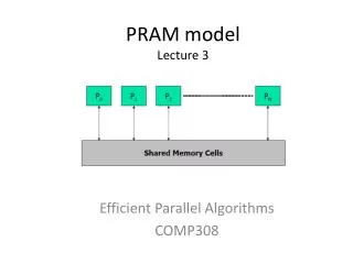
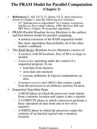
The PRAM Model for Parallel Computation
References • Selim Akl, Parallel Computation: Models and Methods, Prentice Hall, 1997, Updated online version available through website. • Selim Akl, The Design of Efficient Parallel Algorithms, Chapter 2 in “Handbook on Parallel and Distributed Processing” edited by J. Blazewicz, K. Ecker, B. Plateau, and D. Trystram, Springer Verlag, 2000. • Selim Akl, Design & Analysis of Parallel Algorithms, Prentice Hall, 1989. • Henri Casanova, Arnaud Legrand, and Yves Robert, Parallel Algorithms, CRC Press, 2009. • Cormen, Leisterson, and Rivest, Introduction to Algorithms, 1st edition (i.e., older), 1990, McGraw Hill and MIT Press, Chapter 30 on parallel algorithms. • Phillip Gibbons, Asynchronous PRAM Algorithms, Ch 22 in Synthesis of Parallel Algorithms, edited by John Reif, Morgan Kaufmann Publishers, 1993. • Joseph JaJa, An Introduction to Parallel Algorithms, Addison Wesley, 1992. • Michael Quinn, Parallel Computing: Theory and Practice, McGraw Hill, 1994 • Michael Quinn, Designing Efficient Algorithms for Parallel Computers, McGraw Hill, 1987.
Outline • Computational Models • Definition and Properties of the PRAM Model • Parallel Prefix Computation • The Array Packing Problem • Cole’s Merge Sort for PRAM • PRAM Convex Hull algorithm using divide & conquer • Issues regarding implementation of PRAM model
Concept of “Model” • An abstract description of a real world entity • Attempts to capture the essential features while suppressing the less important details. • Important to have a model that is both precise and as simple as possible to support theoretical studies of the entity modeled. • If experiments or theoretical studies show the model does not capture some important aspects of the physical entity, then the model should be refined. • Some people will not accept most abstract model of reality, but instead insist on reality. • Sometimes reject a model as invalid if it does not capture every tiny detail of the physical entity.
Parallel Models of Computation • Describes a class of parallel computers • Allows algorithms to be written for a general model rather than for a specific computer. • Allows the advantages and disadvantages of various models to be studied and compared. • Important, since the life-time of specific computers is quite short (e.g., 10 years).
Controversy over Parallel Models • Some professionals (often engineers) will not accept a parallel model if • It does not capture every detail of reality • It cannot currently be built • Engineers often insist that a model must be valid for any number of processors • Parallel computers with more processors than the number of atoms in the observable universe are unlikely to be built in the foreseeable future. • If they are ever built, the model for them is likely to be vastly different from current models today. • Even models that allow a billion or more processors are likely to be very different from those supporting at most a few million processors.
The PRAM Model • PRAM is an acronym for Parallel Random Access Machine • The earliest and best-known model for parallel computing. • A natural extension of the RAM sequential model • More algorithms designed for PRAM than any other model.
The RAM Sequential Model • RAM is an acronym for Random Access Machine • RAM consists of • A memory with M locations. • Size of M can be as large as needed. • A processor operating under the control of a sequential program which can • load data from memory • store date into memory • execute arithmetic & logical computations on data. • A memory access unit (MAU) that creates a path from the processor to an arbitrary memory location.
RAM Sequential Algorithm Steps • A READ phase in which the processor reads datum from a memory location and copies it into a register. • A COMPUTE phase in which a processor performs a basic operation on data from one or two of its registers. • A WRITE phase in which the processor copies the contents of an internal register into a memory location.
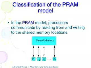
PRAM Model Discussion • Let P1, P2 , ... , Pn be identical processors • Each processor is a RAM processor with a private local memory. • The processors communicate using m shared (or global) memory locations, U1, U2, ..., Um. • Allowing both local & global memory is typical in model study. • Each Pi can read or write to each of the m shared memory locations. • All processors operate synchronously (i.e. using same clock), but can execute a different sequence of instructions. • Some authors inaccurately restrict PRAM to simultaneously executing the same sequence of instructions (i.e., SIMD fashion) • Each processor has a unique index called, the processor ID, which can be referenced by the processor’s program. • Often an unstated assumption for a parallel model
PRAM Computation Step • Each PRAM step consists of three phases, executed in the following order: • A read phase in which each processor may read a value from shared memory • A compute phase in which each processor may perform basic arithmetic/logical operations on their local data. • A write phase where each processor may write a value to shared memory. • Note that this prevents reads and writes from being simultaneous. • Above requires a PRAM step to be sufficiently long to allow processors to do different arithmetic/logic operations simultaneously.
SIMD Style Execution for PRAM • Most algorithms for PRAM are of the single instruction stream multiple data (SIMD) type. • All PEs execute the same instruction on their own datum • Corresponds to each processor executing the same program synchronously. • PRAM does not have a concept similar to SIMDs of all active processors accessing the ‘same local memory location’ at each step.
SIMD Style Execution for PRAM(cont) • PRAM model was historically viewed by some as a shared memory SIMD. • Called a SM SIMD computer in [Akl 89]. • Called a SIMD-SM by early textbook [Quinn 87]. • PRAM executions required to be SIMD [Quinn 94] • PRAM executions required to be SIMD in [Akl 2000]
The Unrestricted PRAM Model • The unrestricted definition of PRAM allows the processors to execute different instruction streams as long as the execution is synchronous. • Different instructions can be executed within the unit time allocated for a step • See JaJa, pg 13 • In the Akl Textbook, processors are allowed to operate in a “totally asychronous fashion”. • See page 39 • Assumption may have been intended to agree with above, since no charge for synchronization or communications is included.
Asynchronous PRAM Models • While there are several asynchronous models, a typical asynchronous model is described in [Gibbons 1993]. • The asychronous PRAM models do not constrain processors to operate in lock step. • Processors are allowed to run synchronously and then charged for any needed synchronization. • A non-unit charge for processor communication. • Take longer than local operations • Difficult to determine a “fair charge” when message-passing is not handled in synchronous-type manner. • Instruction types in Gibbon’s model • Global Read, Local operations, Global Write, Synchronization • Asynchronous PRAM models are useful tools in study of actual cost of asynchronous computing • The word ‘PRAM’ usually means ‘synchronous PRAM’
Some Strengths of PRAM Model JaJa has identified several strengths designing parallel algorithms for the PRAM model. • PRAM model removes algorithmic details concerning synchronization and communication, allowing designers to focus on obtaining maximum parallelism • A PRAM algorithm includes an explicit understanding of the operations to be performed at each time unit and an explicit allocation of processors to jobs at each time unit. • PRAM design paradigms have turned out to be robust and have been mapped efficiently onto many other parallel models and even network models.
PRAM Strengths (cont) • PRAM strengths - Casanova et. al. book. • With the wide variety of parallel architectures, defining a precise yet general model for parallel computers seems hopeless. • Most daunting is modeling of data communications costs within a parallel computer. • A reasonable way to accomplish this is to only charge unit cost for each data move. • They view this as ignoring computational cost. • Allows minimal computational complexity of algorithms for a problem to be determined. • Allows a precise classification of problems, based on their computational complexity.
PRAM Memory Access Methods • Exclusive Read(ER): Two or more processors can not simultaneously read the same memory location. • Concurrent Read (CR): Any number of processors can read the same memory location simultaneously. • Exclusive Write (EW): Two or more processors can not write to the same memory location simultaneously. • Concurrent Write (CW): Any number of processors can write to the same memory location simultaneously.
Variants for Concurrent Write • Priority CW: The processor with the highest priority writes its value into a memory location. • Common CW: Processors writing to a common memory location succeed only if they write the same value. • Arbitrary CW: When more than one value is written to the same location, any one of these values (e.g., one with lowest processor ID) is stored in memory. • Random CW: One of the processors is randomly selected write its value into memory.
Concurrent Write (cont) • Combining CW: The values of all the processors trying to write to a memory location are combined into a single value and stored into the memory location. • Some possible functions for combining numerical values are SUM, PRODUCT, MAXIMUM, MINIMUM. • Some possible functions for combining boolean values are AND, INCLUSIVE-OR, EXCLUSIVE-OR, etc.
ER & EW Generalizations • Casanova et.al. mention that sometimes ER and EW are generalized to allow a bounded number of read/write accesses. • With EW, the types of concurrent writes must also be specified, as in CW case.
Additional PRAM comments • PRAM encourages a focus on minimizing computation and communication steps. • Means & cost of implementing the communications on real machines ignored • PRAM is often considered as unbuildable & impractical due to difficulty of supporting parallel PRAM memory access requirements in constant time. • However, Selim Akl shows a complex but efficient MAU for allPRAM models (EREW, CRCW, etc) that can be supported in hardware in O(lg n) time for n PEs and O(n) memory locations. (See [2. Ch.2]. • Akl also shows that the sequential RAM model also requires O(lg m) hardware memory access time for m memory locations. • Some strongly criticize PRAM communication cost assumptions but accept without question the cost in RAM memory cost assumptions.
Parallel Prefix Computation • EREW PRAM Model is assumed for this discussion • A binary operation on a set S is a function :SS S. • Traditionally, the element (s1, s2) is denoted as s1s2. • The binary operations considered for prefix computations will be assumed to be • associative: (s1 s2) s3 = s1 (s2 s3 ) • Examples • Numbers: addition, multiplication, max, min. • Strings: concatenation for strings • Logical Operations: and, or, xor • Note: is not required to be commutative.
Prefix Operations • Let s0, s1, ... , sn-1 be elements in S. • The computation of p0, p1, ... ,pn-1 defined below is called prefixcomputation: p0 = s0 p1 = s0 s1 . . . pn-1= s0 s1 ... sn-1
Prefix Computation Comments • Suffix computation is similar, but proceeds from right to left. • A binary operation is assumed to take constant time, unless stated otherwise. • The number of steps to compute pn-1 has a lower bound of (n) since n-1 operations are required. • Next visual diagram of algorithm for n=8 from Akl’s textbook. (See Fig. 4.1 on pg 153) • This algorithm is used in PRAM prefix algorithm • The same algorithm is used by Akl for the hypercube (Ch 2) and a sorting combinational circuit (Ch 3).
EREW PRAM Prefix Algorithm • Assume PRAM has n processors, P0, P1 , ... , Pn-1, and n is a power of 2. • Initially, Pi stores xi in shared memory location si for i = 0,1, ... , n-1. • Algorithm Steps: for j = 0 to (lg n) -1, do for i = 2j to n-1 in parallel do h = i - 2j si= sh si endfor endfor
Prefix Algorithm Analysis • Running time is t(n) = (lg n) • Cost is c(n) = p(n) t(n) =(n lg n) • Note not cost optimal, as RAM takes (n)
Example for Cost Optimal Prefix • Sequence – 0,1,2,3,4,5,6,7,8,9,10,11,12,13,14,15 • Use n / lg n PEs with lg(n) items each • 0,1,2,3 4,5,6,7 8,9,10,11 12,13,14,15 • STEP 1: Each PE performs sequential prefix sum • 0,1,3,6 4,9,15,22 8,17,27,38 12,25,39,54 • STEP 2: Perform parallel prefix sum on last nr. in PEs • 0,1,3,6 4,9,15,28 8,17,27,66 12,25,39,120 • Now prefix value is correct for last number in each PE • STEP 3: Add last number of each sequence to incorrect sums in next sequence (in parallel) • 0,1,3,6 10,15,21,28 36,45,55,66 78,91,105,120
A Cost-Optimal EREW PRAM Prefix Algorithm • In order to make the prefix algorithm optimal, we must reduce the cost by a factor of lg n. • We reduce the nr of processors by a factor of lg n (and check later to confirm the running time doesn’t change). • Let k = lg n and m = n/k • The input sequence X = (x0, x1, ..., xn-1) is partitioned into m subsequences Y0, Y1 , ... ., Ym-1 with k items in each subsequence. • While Ym-1 may have fewer than k items, without loss of generality (WLOG) we may assume that it has k items here. • Then all sequences have the form, Yi = (xi*k, xi*k+1, ..., xi*k+k-1)
PRAM Prefix Computation(X, ,S) • Step 1: For 0 i < m, each processor Picomputes the prefix computation of the sequence Yi= (xi*k, xi*k+1, ..., xi*k+k-1) using the RAM prefix algorithm (using ) and stores prefix results as sequence si*k, si*k+1, ... , si*k+k-1. • Step 2: All m PEs execute the preceding PRAM prefix algorithm on the sequence (sk-1, s2k-1 , ... , sn-1) • Initially Piholds si*k-1 • Afterwards Piplaces the prefix sum sk-1 ... sik-1 in sik-1 • Step 3: Finally, all Pi for 1im-1 adjust their partial value sums for all but the final term in their partial sum subsequence by performing the computation sik+j sik+j sik-1 for 0 j k-2.
Algorithm Analysis • Analysis: • Step 1 takes O(k) = O(lg n) time. • Step 2 takes (lg m) = (lg n/k) = O(lg n- lg k) = (lg n - lg lg n) = (lg n) • Step 3 takes O(k) = O(lg n) time • The running time for this algorithm is (lg n). • The cost is ((lg n) n/(lg n)) = (n) • Cost optimal, as the sequential time is O(n) • The combined pseudocode version of this algorithm is given on pg 155 of the Akl textbook
The Array Packing Problem • Assume that we have • an array of n elements, X = {x1, x2, ... , xn} • Some array elements are marked (or distinguished). • The requirements of this problem are to • pack the marked elements in the front part of the array. • place the remaining elements in the back of the array. • While not a requirement, it is also desirable to • maintain the original order between the marked elements • maintain the original order between the unmarked elements
A Sequential Array Packing Algorithm • Essentially “burn the candle at both ends”. • Use two pointers q (initially 1) and r (initially n). • Pointer q advances to the right until it hits an unmarked element. • Next, r advances to the left until it hits a marked element. • The elements at position q and r are switched and the process continues. • This process terminates when q r. • This requires O(n) time, which is optimal. (why?) Note: This algorithm does not maintain original order between elements
EREW PRAM Array Packing Algorithm • Set si in Pi to 1 if xi is marked and set si = 0 otherwise. 2. Perform a prefix sum on S =(s1, s2 ,..., sn) to obtain destination di = si for each marked xi . 3. All PEs set m = sn , the total nr of marked elements. 4. Pi sets si to 0 if xi is marked and otherwise sets si = 1. 5. Perform a prefix sum on S and set di = si + m for each unmarked xi . 6. Each Pi copies array element xi into address di in X.
Array Packing Algorithm Analysis • Assume n/lg(n) processors are used above. • Optimal prefix sums requires O(lg n) time. • The EREW broadcast of sn needed in Step 3 takes O(lg n) time using either • a binary tree in memory (See Akl text, Example 1.4.) • or a prefix sum on sequence b1,…,bn with b1= an and bi= 0 for 1< i n) • All and other steps require constant time. • Runs in O(lg n) time, which is cost optimal. (why?) • Maintains original order in unmarked group as well Notes: • Algorithm illustrates usefulness of Prefix Sums There many applications for Array Packing algorithm. Problem: Show how a PE can broadcast a value to all other PEs in EREW in O(lg n) time using a binary tree in memory.
List Ranking Algorithm(Using Pointer Jumping) • Problem: Given a linked list, find the location of each node in the list. • Next algorithm uses the pointer jumping technique • Ref: Pg 6-7 Casanova, et.al. & Pg 236-241 Akl text. In Akl’s text, you should read prefix sum on pg 236-8 first. • Assume we have a linked list L of n objects distributed in PRAM’s memory • Assume that each Pi is in charge of a node i • Goal: Determine the distance d[i] of each object in linked list to the end, where d is defined as follows: 0 if next[i] = nil d[i] = d[next [i]] +1 if next[i] ≠ nil
Potential Problems? • Consider following steps: • d[i] = d[i] + d[next[i+1]] • next[i] = next[next[i]] • Casanova, et.al, pose below problem in Step7 • Pi reads d[i+1]and uses this value to update d[i] • Pi-1 must read d[i] to update d[i-1] • Computation fails if Pi change the value of d[i] before Pi-1 can read it. • This problem should not occur, as all PEs in PRAM should execute algorithm synchronously. • The same problem is avoided in Step 8 for the same reason
Potential Problems? (cont.) • Does Step 7 (&Step 8) require CR PRAM? d[i] = d[i] + d[next[i]] • Let j = next[i] • Casanova et.al. suggests that Pi and Pj may try to read d[j] concurrently, requiring a CR PRAM model • Again, if PEs are stepping through the computations synchronously, EREW PRAM is sufficient here • In Step 4, PRAM must determine whether there is a node i with next[i] ≠ nil. A CWCR solution is: • In Step 4a, set done to false • In Step 4b, all PE write boolean value of “next[i] = nil” using CW-common write. • A EREW solution for Step 7 is given next
Rank-Computation using EREW • Theorem: The Rank-Computation algorithm only requires EREW PRAM • Replace Step 4 with • For step = 1 to log n do, • Akl raises the question of what to do if an unknown number of processors Pi, each of which is in charge of node i (see pg 236). • In this case, it would be necessary to go back to the CRCW solution suggested earlier.
PRAM Model Separation • We next consider the following two questions • Is CRCW strictly more powerful than CREW • Is CREW strictly more powerful that EREW • We can solve each of above questions by finding a problem that the leftmost PRAM can solve faster than the rightmost PRAM
CRCW Maximum Array Value Algorithm CRCW Compute_Maximum (A,n) • Algorithm requires O(n2) PEs, Pi,j. • forall i {0, 1, … , n-1} in parallel do • Pi,0 sets m[i] = True • forall i, j {0, 1, … , n-1}2, i≠j, in parallel do • [if A[i] < A[j] then Pi,jsets m[i] = False • forall i {0, 1, … , n-1} in parallel do • If m[i] = True, then Pi,0sets max = A[i] • Return max • Note that on n PEs do EW in steps 1 and 3 • The write in Step 2 can be a “common CW” • Cost is O(1) O(n2) which is O(n2)
CRCW More Powerful Than CREW • The previous algorithm establishes that CRCW can calculate the maximum of an array in O(1) time • Using CREW, only two values can be merged into a single value by one PE in a single step. • Therefore the number of values that need to be merged can be halved at each step. • So the fastest possible time for CREW is (log n)
CREW More Powerful Than EREW • Determine if a given element e belongs to a set {e1, e2, … , en} of n distinct elements • CREW can solve this in O(1) using n PEs • One PE initializes a variable result to false • All PEs compare e to one ei. • If any PE finds a match, it writes “true” to result. • On EREW, it takes (log n) steps to broadcast the value of e to all PEs. • The number of PEs with the value of e can be doubled at each step.
Simulating CRCW with EREW Theorem: An EREW PRAM with p PEs can simulate a common CRCW PRAM with p PEs in O(log p) steps using O(p) extra memory. • See Pg 14 of Casanova, et. al. • The only additional capabilities of CRCW that EREW PRAM has to simulate are CR and CW. • Consider a CW first, and initially assume all PE participate. • EREW PRAM simulates this CW by creating a p2 array A with length p
Simulating Common CRCW with EREW • When a CW write is simulated, PRAM EREW PE j writes • The memory cell address wishes to write to in A(j,0) • The value it wishes into memory in A(j,1). • If any PE j does not participate in CW, it will write -1 to A(j,0). • Next, sort A by its first column. This brings all of the CW to same location together. • If memory location in A(0,1) is not -1, then PE 0 writes the data value in A(0,1) to memory location value stored in A(0,1).
PRAM Simulations (cont) • All PEs j for j>0 read memory address in A(j,0) and A(j-1,0) • If memory location in A(j,0) is -1, PE j does not write. • Also, if the two memory addresses are the same, PE j does not write to memory. • Otherwise, PE j writes data value in A(j,1) to memory location in A(j,0). • Cole’s algorithm that EREW can sort n items in log(n) time is needed to complete this proof. It is discussed next in Casanova et.al. for CREW. Problem: • This proof is invalid for CRCW versions stronger than common CRCW, such as combining.