Download
1 / 48
480 likes | 492 Vues
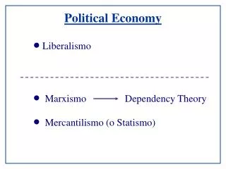
Political Economy: Evolutionary Economics. Complexity & self-organisation. Recap. Veblen & Schumpeter: two different directions for evolutionary economics Veblen: anti-neoclassical statics must be abandoned; but no model Schumpeter: pro-neoclassical

E N D
Political Economy: Evolutionary Economics Complexity & self-organisation
Recap • Veblen & Schumpeter: two different directions for evolutionary economics • Veblen: anti-neoclassical • statics must be abandoned; • but no model • Schumpeter: pro-neoclassical • statics can co-exist with disequilibrium transformational growth; • a model • Modern evolutionary political economy combines V&B: • Veblenian rejection of (neoclassical) statics • Schumpeterian model of transformational growth
Why the hybrid? • Incompatibility of static & dynamic/evolutionary reasoning • Neoclassical economists tend to think: • “Evolution leads to optimising behaviour” • “Dynamics explains movement from one equilibrium point to another” • So “statics is long run dynamics” • also believed by Sraffian economists • implicit in Post Keynesian or Marxian analysis using comparative static or simultaneous equation methods Statics Dynamics Evolution
Why the hybrid? • Modern mathematics reverses this • Field of evolution larger than dynamics • Dynamics larger than statics • Results of evolutionary analysis more general than dynamics • But two generally consistent • Results of dynamics more general than statics • & GENERALLY INCONSISTENT • Dynamic results correct if actual system dynamic/evolutionary Evolution Dynamics Statics • An example: supply and demand analysis
Supply & Demand Analysis • Typical supply & demand exercise: • Demand a decreasing linear function of quantity • Supply an increasing linear function of quantity • Equate the two to find equilibrium Q & P: • Two equations return same result…
Supply & Demand Analysis • An example: • D(Q)=1000-2/10000000 Q • S(Q)=-100+1/10000000 Q
Supply & Demand Analysis • “X” marks the spot! • (Are neoclassical economists really just frustrated pirates?…)
Supply & Demand Analysis • What if initial price isn’t equilibrium price; how does it get there? • Dynamic analysis • Demand price and supply price as functions of time • Producers plan output based on last year’s prices • Consumers react to today’s prices • Convergence to equilibrium over time…
Supply & Demand Analysis • Confirming that this gives the same result as static analysis • Try with initial quantity 10% more than Qe:
Supply & Demand Analysis • Convergence • So “Statics is long run dynamics”? • Let’s try another demand & supply pair…
Supply & Demand Analysis • D(Q)=1000+5/100000000 Q • S(Q)=-100+1/10000000 Q • Meaningful (non-negative) equilibrium price & quantity as before • The dynamic answer…?
Dynamic Instability • Whoops! • Quantity unstable • Cause: slope of supply curve steeper than demand • But also unrealistic: negative quantities • Dynamic model must be wrong then?…
Dynamic Instability • Model of single Market • Converges to equilibrium if b>d • Consumers’ more responsive than suppliers • Diverges from equilibrium if b<d • Suppliers more responsive than consumers • Two possibilities • Either consumers are more volatile than suppliers • Contradicted by the data • Or the model is wrong somehow… • Similar debate occurred in IS-LM modelling:
Dynamic Instability • Hicks (father of IS-LM analysis) on instability • Harrod “welcomes the instability of his system, because he believes it to be an explanation of the tendency to fluctuation which exists in the real world. I think, as I shall proceed to show, that something of this sort may well have much to do with the tendency to fluctuation. But mathematical instability does not in itself elucidate fluctuation. A mathematically unstable system does not fluctuate; it just breaks down. The unstable position is one in which it will not tend to remain.” (Hicks 1949) • I.e., “models must have stable equilibria”3
Dynamic Instability • Kaldor analysed dynamics of IS-LM model • Stable if “slope of S”> “slope of I” • “any disturbances … would be followed by the re-establishment of a new equilibrium, … this … assumes more stability than the real world, in fact, appears to possess.” (80) • Unstable if “slope of I”> “slope of S” • “the economic system would always be rushing either towards a state of hyper-inflation … or towards total collapse… this possibility can be dismissed” (80) • “Since thus neither of these two assumptions can be justified, we are left with the conclusion that the I and S functions cannot both be linear.” (81) • I.e. “models must have nonlinear functions”
Dynamic Instability • 1st set of insights not known to Schumpeter • Simple (non-evolutionary) models of market can fail to converge to equilibrium under realistic conditions (suppliers more responsive than consumers, investors more responsive than savers) • Models can have unstable dynamics and not break down if functions nonlinear • Underlying static partial equilibrium model need not converge to equilibrium… • What about general equilibrium? • 2nd insight not known to Schumeter (or many economists today!) • General “equilibrium” is unstable
Dynamic Instability • Schumpeter’s faith in equilibrium tendency of non-evolutionary markets derived from Walras • Walras believed market system would find equilibrium prices and quantities by“tatonnement” (“groping”) process • Start with randomly chosen starting point • Adjust prices iteratively • Increase price where demand > supply • Decrease price where demand < supply • Converge to equilibrium prices & quantities • In Walras’ words…
Dynamic Instability • “Once the prices … have been cried at random…, each party … will offer … those goods or services of which he thinks he has relatively too much, and he will demand those articles of which he thinks he has relatively too little … the prices of those things for which the demand exceeds the offer will rise, and the prices of those things of which the offer exceeds the demand will fall. New prices now having been cried, each party to the exchange will offer and demand new quantities. And again prices will rise or fall until the demand and the offer of each good and each service are equal…” (Walras 1874) • Convergence to general equilibrium over time?
General Disequilibrium • General equilibrium requires stable output & prices • Yt= Yt-1 = Ye (or with growth) Yt= (1+g) Yt-1 • Where Y = vector of all commodities in economy • Pt = Pt-1 = Pe • Where P = vector of relative prices of all commodities in economy • Constant relative prices • Modern maths shows these two inconsistent… • Either prices stable & quantities unstable, or • prices unstable & quantities stable • But not both (Jorgenson ‘60,61; McManus ‘63, Blatt ’83) • So “general equilibrium” will never converge to equilibrium, so that…
General Disequilibrium • ‘There exist known systems, therefore, in which the important and interesting features of the system are “essentially dynamic”, in the sense that they are not just small perturbations around some equilibrium state, perturbations which can be understood by starting from a study of the equilibrium state and tacking on the dynamics as an afterthought.’ • ‘If it should be true that a competitive market system is of this kind, then… No progress can then be made by continuing along the road that economists have been following for 200 years. The study of economic equilibrium is then little more than a waste of time and effort…’ Blatt (1983: 5-6)
General Dynamics • Schumpeter’s evolutionary economics was done by “starting from a study of the equilibrium state and tacking on evolution as an afterthought” • We now know this can’t be done • So modern evolutionary economics • Veblenian anti-equilibrium, Schumpeterian models • Builds dynamic models & add evolution later; or • Builds evolutionary models from the outset • Former approach more common • Easier (potentially dangerous reason!) • Can incorporate “vision” of given economic theory (Marx, Keynes,…) • Close match to slowly evolving systems • Insights from complex systems to evolution
In summary… • Summarising validity of analytic techniques & relations between them: • Now insights on evolution from complex systems…
Complexity & Evolution… • Previous supply & demand model “linear” • Variables added together • Only variables and constants • Kaldor’s insight—real world cannot be this simple • Variables must interact in more complex ways than simple addition • Models with nonlinear relations between variables generate complex behaviour from even “simple” models • Two examples • Discrete logistic model of population • Lorenz’s “quasi-quadratic” weather model
Complexity & Evolution… • Logistic population model • Simplest population model is: • This year’s population • Equals last year’s • Multiplied by growth rate • Model predicts population grows to infinity • But real-world populations will hit constraints • Simplest constraint • Cow tramples grass another cow could have eaten • Interaction reduces life expectancy • Interaction function of number of animals squared:
Complexity & Evolution… • Ratio a/b gives “equilibrium” population • For b=0, exponential growth of population forever:
Complexity & Evolution… • For b>0, population first rises at accelerating rate and then slowly tapers to equilibrium level:
Complexity & Evolution… • For a=2 (2 births per animal per cycle), a “2-cycle” results • Population overshoots carrying capacity • Interactions reduce population to below carrying capacity • And so on forever…
Complexity & Evolution… • For a>2.7, chaos • Population bounces around in unpredictable way • Cycles never quite repeat (aperiodic) but never cease either • But behind the apparent disorder, structure—hence “complexity” rather than “chaos” theory
Complexity & Evolution… • Another example: Lorenz’s weather model: simple system 3 equations, 3 unknowns, 3 constants… • Just 2 semi-quadratic nonlinear terms z.x and x.y x displacement y displacement temperature gradient • Model has 3 equilibria • All 3 are unstable • Generates incredibly complex cycles that are • Highly sensitive to initial conditions; but • Have underlying common structure
Complexity & Evolution… • x,y,z values bounce around like crazy…
Complexity & Evolution… • Small change in initial conditions has huge impact on eventual system path
Complexity & Evolution… • Behind the apparent chaos, an incredibly intricate structure… • Basic feature: system never even approaches equilibria Equilibrium 2 Equilibrium 1 Equilibrium 3
Complexity & Evolution… • Equilibrium highly unstable: start just next to it and get propelled away instantly… • Strange role of equilibria in nonlinear dynamics/evolution… Start near equilibrium 3
Complexity & Evolution… • Systems almost always have unstable equilibria • Many technical ways to measure degree of stability of dynamic system • Dominant eigenvalue, Lyupanov exponent, Hurst exponent,… • Basic idea of all measures: • Greater than one value, system diverges from equilibrium (eigenvalue) • Greater than another, initial starting points spread apart in time—“sensitive dependence on initial conditions”, “butterfly effect” • Greater than another, system inherently unstable: fluctuations not only due to random shocks but also inherent instability of system feedbacks
“Edge of chaos”… • Fixed dynamic system like Logistic is either one side or the other of measures • Dominant eigenvalue < 1, stable equilibrium • Dominant eigenvalue > 1, unstable equilibrium • Lyapunov exponent > 1, chaos • Evolutionary systems (e.g., when parameters a & b can change over time) tend to “the edge of chaos” • System oscillates between stability and chaos • Small change in parameters either way shift from stable to unstable and vice versa. • Living systems appear to dynamic systems that evolve to “edge of chaos” • Other insights from complexity analysis
“Emergent behaviour”… • Group behaviour occurs that is not predictable from properties of individuals in it but depends on relationships between them • Relationships may evolve as much as individuals • E.g., individual sparrows easily fall prey to Hawk • Sparrows that fly together increase chances of survival • Relationship of flying together evolves • “Flocking” results • Intuitions • Macro outcomes can be very different to micro level behaviour • Similar conclusion reached by some neoclassicals…
“Emergent behaviour”… • Failure to derive coherent market demand curves from individual demand curves led to conclusion that… • ‘If we are to progress further we may well be forced to theorise in terms of groups who have collectively coherent behaviour. Thus demand and expenditure functions if they are to be set against reality must be defined at some reasonably high level of aggregation. The idea that we should start at the level of the isolated individual is one which we may well have to abandon.’ (Kirman 1989)
Dynamic & Evolutionary Modelling • Dynamic modelling mature field • Mathematical techniques well-known • Computer simulation tools sophisticated • Evolutionary modelling relatively immature • No mathematical tools • Computer simulation tools complicated to use • Basic methods in both • Specify characteristics of entities • Specify relationships between entities • Specify adaptive processes • change in number, size of entities
Dynamic & Evolutionary Modelling • Differences • Dynamic modelling • Behaviour of entities remains constant • Parameters of relationships remain constant • Evolutionary modelling • Behaviour alters via mutation/adaptation • Parameters of relationships alter
Dynamic & Evolutionary Modelling • Basic tools of dynamic modelling • System of difference equations • Property now = some nonlinear function of properties in previous time period • System of differential equations • Rate of change of property now = nonlinear function of properties now (or lagged) • Differential equations more general • Approximate behaviour of large numbers • Discrete technical change by each firm sums to near continuous technical change by industry…
Dynamic & Evolutionary Modelling • Final, “closed form” solutions can’t be specified • With equilibrium comparative statics, can conclude, e.g.: • With single differential equation, can conclude, e.g.: • With 3 or more coupled nonlinear differential equations • No closed form solution exists • Must simulate… • On which, advanced dynamic tools…
Dynamic & Evolutionary Modelling • Advanced tools… • Specialised mathematical programs • Mathcad, Mathematica, Matlab, Maple… • Much more powerful, flexible than spreadsheets… • Flowchart tools Simulink, Vissim, IThink • E.g., stockmarket model…
Dynamic & Evolutionary Modelling • Stock market with fundamental trades, bandwagons, collective optimism/pessimism & panics: Matlab/Simulink
Dynamic & Evolutionary Modelling • Contra Efficient Markets Hypothesis, model generates realistic bull/bear cycles, crashes… • But no alteration of behaviour over time • Sufficient for description of systemic dynamics • Insufficient for evolution of individual & systemic behaviour over time…
Dynamic & Evolutionary Modelling • Evolutionary modelling • Entities and relationships specified • at individual level (“agents”) • in discrete form (aggregation gives collective emergent behaviour) • Adaptive formula for change in parameters of entities/relationships specified • Parameters altered adaptively each time step • Sometimes • Rules for “death”, “crossover”, “mutation” • Spontaneous appearance of new entities (products, firms) • Only feasible tool at present computer programming • On which, more next week!
References Blatt, J.M., (1983). Dynamic Economic Systems, ME Sharpe, Armonk. Hicks, J.R., (1949). “Mr Harrod’s Dynamics”, Economic Journal: 68-75 Jorgenson, D. W., (1961). “Stability of a dynamic input-output system”, Review of Economic Studies 28: 105-116. “Stability of a dynamic input-output system: a reply”, Review of Economic Studies 30: 148-149. Kaldor, N., (1940). “A model of the trade cycle”, Economic Journal: 78-92 Kirman, A., (1989). “The intrinsic limits of modern economic theory—the emperor has no clothes”, Economic Journal 99: 126-139. McManus, M., (1963), “Notes on Jorgenson's Model”, Review of Economic Studies 30: 141-147. Walras, L., (1874). Elements of Pure Economics, Augustus M Kelley, Farfield
General Disequilibrium • Most basic model of production is input-output • “It takes ½ ton of steel and 5 tons of coal to make 1 ton of steel…” etc. • Can be represented as matrix equation • Yt=A Yt-1 • Where A is matrix of input-output coefficients • Single number can be derived from A: • Yt= l Yt-1 • Just like Yt=(1+g) Yt-1