Download
1 / 28
280 likes | 485 Vues
Simulation of single phase reactive transport on pore-scale images. Zaki Al Nahari, Branko Bijeljic, Martin Blunt. Outline. Motivation Modelling reactive transport Geometry & flow field Transport Reaction rate Validation against analytical solutions Results Future work. Motivation.

E N D
Simulation of single phase reactive transport on pore-scale images Zaki Al Nahari, Branko Bijeljic, Martin Blunt
Outline • Motivation • Modelling reactive transport • Geometry & flow field • Transport • Reaction rate • Validation against analytical solutions • Results • Future work
Motivation • Contaminant transport: • Industrial waste • Biodegradation of landfills…etc • Carbon capture and storage: • Acidic brine. • Over time, potential dissolution and/or mineral trapping. • However…. • Uncertainty in reaction rates • The field <<in the lab. • No fundamental basis to integrate flow, transport and reaction in porous media.
Geometry & Flow • Micro-CT scanner uses X-rays to produce a sequence of cross-sectional tomography images of rocks in high resolution (µm) • To obtain the pressure and velocity field at the pore-scale, the Navier-Stokes equations are fundamental approach for the flow simulation. • Momentum balance • Mass balance • For incompressible laminar flow, Stokes equations can be used: Pore space Velocity field Pressure field
Transport • Track the motion of particles for every time step by: • Advection along streamlines using a novel formulation accounting for zero flow at solid boundaries. It is based on a semi-analytical approach: no further numerical errors once the flow is computed at cell faces. • Diffusion using random walk. It is a series of spatial random displacements that define the particle transitions by diffusion.
Reaction Rate • Bimolecular reaction • A + B → C • The reaction occurs if two conditions are met: • Distance between reactant is less than or equal the diffusive step ( ) • If there is more than one possible reactant, the reaction will be with nearest reactant.. • The probability of reaction (P) as a function of reaction rate constant (k):
Validation for bulk reaction • Reaction in a bulk system against the analytical solution: • no porous medium • no flow • Analytical solution for concentration in bulk with no flow. • Number of Voxels: • Case 1: 10×10×10 • Case 2: 20×20×20 • Case 3: 50×50×50 • Number of particles: • A= 100,000 density= 0.8 Np/voxel • B= 50,000 density= 0.4 Np/voxel • Parameters: • Dm= 7.02x10⁻¹¹ m2/s • k= 2.3x10⁹ M-1.s-1 • Time step sizes: • Δt= 10-3 s P= 3.335×10⁻³ • Δt= 10-4 s P= 1.055×10⁻² • Δt= 10-5 s P= 3.335×10⁻²
Case 1: Number of Voxels= 10×10×10 Δt= 10-3 s Δt= 10-4 s Δt= 10-5 s
Case 2: Number of Voxels= 20×20×20 Δt= 10-3 s Δt= 10-4 s Δt= 10-5 s
Case 3: Number of Voxels= 50×50×50 Δt= 10-3 s Δt= 10-4 s
Results for reactive transport • Berea Sandstone • Number of Voxels: 300×300×300 • Number of particles: • A= 400,000 density= 1.481×10⁻² Np/voxel • B= 200,000 density= 7.407×10⁻³ Np/voxel • Pe= 200 • Case 1: Parallel injection • Both reactants (A and B) injected at the top and bottom half of the inlet. • Case 2: Injection • Reactant, A, is resident in the pore space, while reactant B is injected at the inlet face.
Results; Case 1 - Parallel injection 2-D 3-D y (μm) x (μm) y (μm) z (μm) x (μm)
Results; Case 1 - Parallel injection after 1 sec 2-D 3-D y (μm) x (μm) C= 1087 y (μm) z (μm) x (μm)
Results; Case 2 - Front injection 2-D 3-D y (μm) x (μm) y (μm) z (μm) x (μm)
Results; Case 2 – Front injection after 1 sec 2-D 3-D y (μm) x (μm) C= 713 y (μm) z (μm) x (μm)
Future Work • Fluid-Fluid interactions • Predict experimental data; Gramling et al. (2002) • Fluid-solid interactions • Dissolution and/or precipitation • Change the pore space geometry and hence the flow field over time Gramling et al. (2002)
Acknowledgements: Dr. Branko Bijeljic and Prof. Martin Blunt Emirates Foundation for funding this project Thank you
Series of Images (0, y, z) (0, y, z) Image Mirror (x, y, z) (x, y, z) (x, y, 0) (0, y, 0) (0, y, 0) (x, y, 0) Image + Mirror (x, 0, z) (0, 0, z) (0, 0, z) (x, 0, z) (0, 0, 0) (x, 0, 0) (0, 0, 0) (x, 0, 0) (0, y, z) (0, y, z) (0, y, z) (x, y, z) (x, y, z) (x, y, z) (0, y, 0) (0, y, 0) (0, y, 0) (2x, y, 0) (2x, y, 0) (2x, y, 0) Number Images Image 1 Image 2 (0, 0, z) (0, 0, z) (0, 0, z) (2x, 0, z) (2x, 0, z) (2x, 0, z) (0, 0, 0) (0, 0, 0) (0, 0, 0) (2x, 0, 0) (2x, 0, 0) (2x, 0, 0)
Model • Couple transport with reactions
Advection • General Pollock’s algorithm with no solid boundaries: • To obtain the velocity at position inside a voxel • To estimate the minimum time for a particle to exit a voxel: • To determine the exit position of a particle in the neighbouring voxel Mostaghimi et al. (2010)
Advection 6 algorithms 3 algorithms 8 algorithms 12 algorithms 3 algorithms 12 algorithms 12 algorithms Mostaghimi et al. (2010)
Transport • Particles Motion: • Advection • Diffusion. • To measure the spreading of particles in porous media • Peclet number Bijeljic and Blunt (2006)
Heterogeneous reactions • Assumption: • Temperature is constant • CO2 is dissolved in brine. • No vaporisation process. • No biogeological reactions • Carbonate dissolution and precipitation kinetic constant rate are taken from Chou et al. (1989).
Heterogeneous reactions • Activity Coefficients are estimated using Harvie-Moller-Weare (HMV) methods (Bethke, 1996).
Heterogeneous reactions • Nigrini (1970) approach are used to estimate diffusion coefficient