Download
1 / 43
620 likes | 1.06k Vues
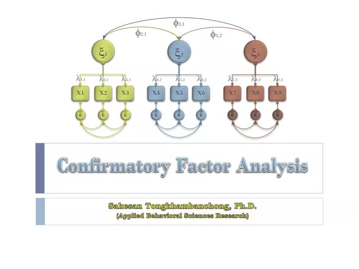
3 ,1. 2,1. 3,2. 1. 2. 3. 1,1. 2,1. 3,1. 4,2. 5,2. 6,2. 7,3. 8,3. 9,3. X1. X2. X3. X4. X5. X6. X7. X8. X9. . . . . . . . . . Confirmatory Factor Analysis. Sakesan Tongkhambanchong, Ph.D. (Applied Behavioral Sciences Research).

E N D
3,1 2,1 3,2 1 2 3 1,1 2,1 3,1 4,2 5,2 6,2 7,3 8,3 9,3 X1 X2 X3 X4 X5 X6 X7 X8 X9 Confirmatory Factor Analysis Sakesan Tongkhambanchong, Ph.D. (Applied Behavioral Sciences Research)
Exploratory vs. Confirmatory Strategies Exploratory Factor Analysis: EFA … it is exploratory in the sense that researchers adopt the inductive strategy of determining the factor structure empirically. (bottom-up Strategy) … researcher allow the statistical procedure to examine the correlations between the variables and to generate a factor structurebased on those relationships. …from the perspective of the researchers at the start of the analysis, any variable may be associated with any component or factor.
Exploratory vs. Confirmatory Strategies Exploratory Factor Analysis: EFA … in EFA the researcher has little or no knowledge about the factor structure regarding: The number of factors or dimensions of the constructs. Whether these dimensions are orthogonal or oblique. The number of indicators of each factor. Which indicators representwhich factor. … there is very little theory that can be used for answering the questions. The researcher may collect data and explore or search for a factor structure or theory which can explain the correlation among the indicators.
An Exploratory Factor Model (EFA) Orthogonal or Oblique (แต่ละองค์ประกอบ มี-ไม่มีความสัมพันธ์กัน) 1 2 3 Factor structure / Component / Dimensions / Unmeasured variables The Factor Loading or the Structure/Pattern Coefficient Measured variables (Observed) / Indicators / Items X1 X2 X3 X4 X5 X6 X7 X8 X9 Errors or Uniqueness May be…3 Factors
An Exploratory Factor Model (EFA) Orthogonal or Oblique (แต่ละองค์ประกอบ มี-ไม่มีความสัมพันธ์กัน) 1 2 Factor structure / Component / Dimensions / Unmeasured variables The Factor Loading or the Structure/Pattern Coefficient Measured variables (Observed) / Indicators / Items X1 X2 X3 X4 X5 X6 X7 X8 X9 Errors or Uniqueness May be…2 Factors
An Exploratory Factor Model (EFA) 1 Factor structure / Component / Dimensions / Unmeasured variables The Factor Loading or the Structure/Pattern Coefficient Measured variables (Observed) / Indicators / Items X1 X2 X3 X4 X5 X6 X7 X8 X9 Errors or Uniqueness Or…may be…1 Factors
An Exploratory Factor Analytic Model (Based on Covariance) A1 A1 A1 A A2 A2 A2 A A3 A3 A3 A4 A4 B1 A5 B1 B2 A B A6 B2 B3 A7 B3 B4 B A8 B4 C1 C C2 A9 B5 C3 A10 B6 One-Factor Model Two-Factor Model Three-Factor Model
Confirmatory Factor Analysis Defined Confirmatory Factor Analysis . . . is similar to EFA in some respects, but philosophically it is quite different. With CFA, the researcher mustspecify both the number of factors that exist within a set of variables and which factor each variable will load highly on before results can be computed.So the technique does not assign variables to factors. Instead the researcher must be able to make this assignment before any results can be obtained. SEM is then applied to test the extent to which a researcher’s a-priori pattern of factor loadings represents the actual data.
Exploratory versus Confirmatory Strategies Confirmatory Factor Analysis: CFA … Confirmatory factor analysis, by contrast, requires researchers to use a deductive strategy.(Top-down Approach) … within this strategy, the factors and the variables that are held to represent them are postulated at the beginning of the procedure rather than emerging from the analysis. … the statistical procedure is then performed to determine how well this hypothesized theoretical structure fits the empirical data.
Exploratory versus Confirmatory Strategies Confirmatory Factor Analysis: CFA … Confirmatory factor analysis, assumes that the structure is known or hypothesized a priori. Ex.Psychological Construct Xis hypothesized as a general factor with three subdimensions or subfactors. Each of these subdimensions is measured by its respective 3-indicators. The indicators are measures of one and only one factor. The complete factor structure along with the respective indicators and the nature of the pattern loadings is specified a priori. …The objective is to empirically verify orconfirmthefactor structure.
Psychological Construct X with 3 subdimensions or subfactors 3,1 2,1 3,2 1 2 3 1,1 2,1 3,1 4,2 5,2 6,2 7,3 8,3 9,3 X1 X2 X3 X4 X5 X6 X7 X8 X9
Objectives of Confirmatory Factor Analysis • Confirmatory Factor Analysis: CFA • Given the sample covariance matrix, to estimate the parameters of the hypothesized factor model. • To determine the fit of the hypothesized factor model. That is, how close is the estimated covariance matrix: , to the sample covariance matrix: S ?
A Confirmatory Factor Analytic Model (CFA)-Based on Theory Some Factors are correlated/ Some Factors are not correlated 3,1 2,1 3,2 1 2 3 Latent Construct Unmeasured variables The Factor Loading or the Structure/Pattern Coefficient 1,1 2,1 3,1 4,2 5,2 6,2 7,3 8,3 9,3 Measured variables (Observed) / Indicators / Items X1 X2 X3 X4 X5 X6 X7 X8 X9 Errors or Uniqueness Some Errors are correlated
An Example of Confirmatory Factor Analysis (CFA) Hypothesized Model of Justice Model Some factors are correlated Some factors are not correlated 3,1 2,1 3,2 1 2 3 1,1 2,1 3,1 4,2 5,2 6,2 7,3 8,3 9,3 10,3 X1 X2 X3 X4 X5 X6 X7 X8 X9 X10 Uniqueness or Error terms are not Independent (correlated)
Confirmatory Factor Analysis Stages Stage 1: Defining Individual Constructs Stage 2: Developing the Overall Measurement Model Stage 3: Designing a Study to Produce Empirical Results Stage 4: Assessing the Measurement Model Validity *Note:CFA involves stages 1 – 4 above. Stage 5: Specifying the Structural Model Stage 6: Assessing Structural Model Validity SEM is stages 1-4 and 5, 6.
A Seven steps process for Analyzing CFA Develop a Theoretically Based Model Final Model Construct a Path Diagram (Factor Model) Model Modification Convert the Path Diagram Model Interpretation Choose the Input Matrix type Evaluate model Goodness-of-fit Correlation matrix Covariance matrix Research Design Issue Assess the Identification of the Model Evaluate model Estimates
An Example of Confirmatory Factor Analysis (CFA) 3,1 2,1 3,2 1 2 3 1,1 2,1 3,1 4,2 5,2 6,2 7,3 8,3 9,3 10,3 X1 X2 X3 X4 X5 X6 X7 X8 X9 X10 Hypothesized Measurement Model (Path Model)
An Example of Confirmatory Factor Analysis (CFA) Last Trimming Model of Justice Model 3,1 = 0.71 2,1 = 0.52 3,2 = 0.47 1 2 3 CR = .782 VE = .473 CR = .823 VE = .540 CR = .600 VE = .449 .62 .71 .72 .68 .79 .92 .67 .70 .75 .81 X1 X2 X3 X4 X5 X6 X7 X8 X9 X10 .482 .616 .496 .538 .370 .160 .550 .510 .440 .340 -.11 .36 .13 .35 Result of Analysis with LISREL program
Alternative Model: Second-order CFA Model Some Factors are correlated/ Some Factors are not correlated 1 Second order Factor 3,1 2,1 3,1 1 2 3 First order Factor 1,1 2,1 3,1 4,2 5,2 6,2 7,3 8,3 9,3 Measured variables (Observed) / Indicators / Items X1 X2 X3 X4 X5 X6 X7 X8 X9 Errors or Uniquenesses Some Errors are correlated
3,1 2,1 3,2 1 2 3 1,1 2,1 3,1 4,2 5,2 6,2 7,3 8,3 9,3 X1 X2 X3 X4 X5 X6 X7 X8 X9 Analysis of CFA with LISREL Sakesan Tongkhambanchong, Ph.D. (Applied Behavioral Sciences Research)
Stage 1: Defining Individual Constructs • List constructs that will comprise the measurement model. • Determine if existing scales/constructs are available or can be modified to test your measurement model. • If existing scales/constructs are not available, then develop new scales.
Hypothesized Measurement Model: Two-Factor model of IQ 1 A 1,1 IQ1 B 2,1 3,1 C D 4,2 IQ2 E 5,2 6,2 F 1 Hypothesized Measurement Model of IQ
Stage 2: Developing the Overall Measurement Model • Key Issues . . . • Unidimensionality – no cross loadings • Congeneric measurement model – no covariance between or within construct error variances • Items per construct – identification • Reflective vs. formative measurement models
CFA Model: Two-Factor model • Congeneric measurement model: Each measured variable is related to exactly one construct 1 Congeneric measurement model: no covariance (correlation) between or within construct error variances A IQ1 B C • Unidimensionality: No cross-loading D IQ2 E F 1 • Reflective measurement models
CFA Model: Two-Factor model with correlate factor 1 A covariance between construct error variances IQ1 B C Cross-loading Covariance within construct error variances D IQ2 E F 1 measurement model is Not Congeneric : Each measured variable is not related to exactly one construct /errors are not independent
Model Identifications: Underidentified, Just-identified & Over-identified 1 1 Parameter estimated = 4 Parameter estimated = 6 2 2 1 1 3 X1 X2 X1 X2 X3 6 4 5 3 4 1 Parameter estimated = 8 1 4 2 3 X1 X2 X3 X4 5 6 7 8
Stage 2: Developing the Overall Measurement Model • Developing the Overall Measurement Model … • In standard CFA applications testing a measurement theory, within and between error covariance terms should be fixed at zero and not estimated. • In standard CFA applications testing a measurement theory, all measured variables should be free to load onlyon one construct. • Latent constructs should be indicated by at least three measured variables, preferably four or more. In other words, latent factors should be statistically identified.
Stage 3: Designing a Study to Produce Empirical Results • The ‘scale’ of a latent construct can be set by either: • Fixing one loading and setting its value to 1, or • Fixing the construct variance and setting its value to 1. • Congeneric, reflective measurement models in which all constructs have at least three item indicators are statistically identified in models with two or more constructs. • The researcher should check for errors in the specification of the measurement model when identification problems are indicated. • Models with large samples (more than 300) that adhere to the three indicator rule generally do not produce Heywood cases.
Stage 4: Assessing Measurement Model Validity • Assessing fit – GOF indices and path estimates (significance and size) • Construct validity • Diagnosing problems • Standardized residuals • Modification indices (MI) • Specification searches
Stage 4: Assessing Measurement Model Validity • Loading estimates can be statistically significant but still be too low to qualify as a good item (standardized loadings below |.5|). In CFA, items with low loadings become candidates for deletion. • Completely standardized loadings above +1.0 or below -1.0 are out of the feasible range and can be an important indicator of some problem with the data. • Typically, standardized residuals less than |2.5| do not suggest a problem. • Standardized residuals greater than |4.0| suggest a potentially unacceptable degree of error that may call for the deletion of an offending item. • Standardized residuals between |2.5| and |4.0| deserve some attention, but may not suggest any changes to the model if no other problems are associated with those items.
Stage 4: Assessing Measurement Model Validity • The researcher should use the modification indices only as a guidelinefor model improvements of those relationships that can theoretically be justified. • CFA results suggesting more than minor modification should be re-evaluated with a new data set (e.g., if more than 20% of the measured variables are deleted, then the modifications can not be considered minor).
Hypothesized Measurement Model:Two-Factor model of IQ 1 1,1 A 1,1 IQ1 2,2 B 2,1 3,1 3,3 C 2,1 4,4 D 4,2 IQ2 5,5 E 5,2 6,2 6,6 F 1 Hypothesized Measurement Model of IQ
Measurement Model of IQ & Data (Input Matrix) • Fitting Models & Data