Download
1 / 12
150 likes | 295 Vues
Exponential Regression. Section 4.1.1. Starter 4.1.1.

E N D
Exponential Regression Section 4.1.1
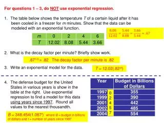
Starter 4.1.1 • The city of Concord was a small town of 10,000 people in 1950. Returning war veterans and the G.I. Bill led to rapid growth which continued through the rest of the 20th century. The table below shows approximate population figures for each decade. • Use linear regression on your calculator to find a mathematical model of the data. HINT: Let x be “years since 1950” instead of calendar years. These are called reference years. • Sketch the scatterplot and LSRL. • Write the equation and the correlation constant. • Sketch the residual plot and comment on how well the LSRL fits the data.
Objectives • Convert exponential data to linear data by use of logarithm principles • Perform linear regression on linearized data • Evaluate linear fit by using a residual plot • Convert linear results to an exponential function of the form y = abx that models the original data
Graphing Activity • Use the special graph paper I give you to graph the Concord growth data. Be sure to label axes. • Put reference year on the x axis • Put population on the y axis • What surprising pattern did you find? • The data are linear • That wasn’t the case in the starter, so why do they appear linear now?
Review of Logarithms • To answer the question, we need to remember some basic facts about logs: • A logarithm is an exponent • So when we ask what is the log of 1000, we mean what exponent could be put over a base of 10 to give a result of 1000? • 103 = 1000, so log 1000 = 3 • Since no base was written, we assume the base is 10 • If we ask what is log28, the answer is 3 because 23=8 • Every exponential statement has an equivalent logarithmic statement • To say 34=81 is equivalent to saying log381=4 • In general, if ab=c, then logac=b • Also: log10x = x and 10log x = x logs & exponents are inverses • Three important rules govern the arithmetic of logs: • Product Rule: log(ab) = log(a) + log(b) • Quotient Rule: log(a/b) = log(a) – log(b) • Power Rule: log(a)b = b log(a)
Applying the Rules of Logs • Consider a general exponential function of the form y=abx where a and b are unknown constants • Suppose we take logs of both sides • log y = log (abx) • log y = log(a) + log(bx) product rule • log y = log (a) + x log(b) power rule • But “a” is just an unknown constant, so log(a) is also an unknown constant that we could call “A” • Similarly, log(b) is a constant that we call “B” • So the last line above could be written: log y = A +Bx • But A + Bx is just a linear function of x • So log y is a linear function of x • That’s why your graph was linear • Notice that your y axis is scaled in log units, so you really graphed x against the log of y, not just y itself.
Finding the LSRL of Linearized Data • Return to the starter data and define L3 to be log(L2) • So L3 contains the logs of the y values in L2 • Set up Plot 2 as a scatterplot of L1 & L3 • Turn off Y1 and Plot 1, then tap zoom-9 to see the linearized data • It should look just like your manual graph • Now perform linear regression of log y against x and paste the LSRL into Y2 • In other words, LinReg(a+bx)L1,L3,Y2 • Note the very high r value of .999 • Tap “GRAPH” to see the fit • Turn off the main graph and turn on the residual plot • Sketch the residual plot • Comment on what the plot says about goodness of fit • Write the equation of the LSRL (round to .001):
Converting from LSRL to Exponential Model • The equation we found says log y = A+Bx • Raise bases of 10 to both sides and simplify • 10log y = 10(A+Bx) • y = 10A 10Bx = (10A)(10B)x • Now recall that A = log a, so 10 A = 10 log a = a • Similarly, 10 B = b • So the equation becomes y = abx • In other words, use LinReg on the linearized data to find A and B, then convert to a and b in the model we seek. • The “magic” formulas are: • To find a, evaluate 10A (where A is the a given by LinReg) • To find b, evaluate 10B (where B is the b given by LinReg)
Finishing the Starter • We previously found A and B in the Concord population problem • A = 4.002 and B = .0211 • So for the exponential model y = abx • a = 104.002 = 10046 • b = 10.0211 = 1.050 • Write the exponential model with the numbers filled in • y = 10046(1.050)x • Put this model in Y3 and graph it with the original data (Plot 1)
Summary • Linear regression on the raw data gave a curved residual plot, so we tried an exponential model instead. • Put logs of y values in L3 and run LinReg. • Check linearized data and resid plot. • Calculator gives A and B, not a and b. • Convert to a and b; enter y = abx and graph on plot of original data.
Objectives • Convert exponential data to linear data by use of logarithm principles • Perform linear regression on linearized data • Evaluate linear fit by using a residual plot • Convert linear results to an exponential function of the form y = abx that models the original data
Homework • Read pages 176 – 188 • Do problem 1