Download

1 / 61
850 likes | 1.69k Vues
TRANSIENT STABILITY STUDIES (POWERTRS). Indonesia Clean Energy Development (ICED) project Indonesia Wind Sector Impact Assessment Presented by: Dr. Balaraman, Ph.D. Makassar, February 17 to 21, 2014. Stability. Transient stability Large disturbance (First swing).

E N D
TRANSIENT STABILITY STUDIES(POWERTRS) Indonesia Clean Energy Development (ICED) project Indonesia Wind Sector Impact Assessment Presented by: Dr. Balaraman, Ph.D. Makassar, February 17 to 21, 2014
Stability Transient stability Large disturbance (First swing) Mid-term/long-term stability Study period: seconds to several minutes (slow dynamics) Rotor angle stability Study period: 0-10 sec Voltage stability Small signal stability Non-oscillatory Insufficient synchronizing torque Oscillatory Unstable control action
Power System Operating States f, v, loading acceptable, load met, n-1 or n-2 contingency acceptable f, v, loading acceptable load met n-1 or n-2 contingency not satisfied f, v, loading not acceptable, load not met
DS: Distribution System G : Generator Control Hierarchy
Power System Stability • Ability of a power system to remain in synchronism • Classification of transients : Electromagnetic and Electromechanical Stability classification • Transient stability : Transmission line faults, sudden load change, loss of generation, line switching etc. • Dynamic stability : Slow or gradual variations. Machine, governor - Turbine, Exciter modelling in detail. • Steady state stability : Changes in operating condition. Simple model of generator.
Assumptions : • Synchronous speed current and voltage are considered. • DC off set currents, harmonics are neglected. • Symmetrical components approach. • Generated voltage is independent of machine speed. • Circuit parameters are constant at nominal system frequency. (Frequency variation of parameter neglected).
Mechanical Equation • J : Moment of inertia of rotor masses (kg-mt2 ) • m : Angular displacement of rotor w.r.t. a stationary axis (mechanical radians) • t : Time (seconds) • Tm : Mechanical or Shaft Torque ( N-m ) • Te : Net electrical torque (N-m ) • Ta : Net accelerating torque (N-m) • For generator, Tm and Te are +ve.
m : Angular displacement of the rotor in mechanical radians.
Where M : Inertia constant = at synchronous speed in Joules-sec per mechanical radian.
Constant is defined as the ratio of stored Kinetic Energy in Mega Joules at synchronous speed and machine rating in MVA
At t = 0, breaker is opened. • Initially Pe = 1 pu on machine rating Pm = 1pu and kept unchanged. • In 2H seconds, the speed doubles.
Inertia constant (H) is in the range 2 - 9 for various types of machines. Hence H-constant is usually defined for machine.
Relation between H constant and Moment of Inertia is given by:
Example : Smach = 1333 MVA, WR2 = 5820000 lb – ft2, N= 1800 RPM = 3.2677575 pu (MJ/ MVA) On 100 MVA base : H = 1333 / 100 = 43.56 (MJ / MVA)
H = H1 + H2 Pm = Pm1 + Pm2 Pe= Pe1 + Pe2 G1 and G2 are called coherent machines. Inertia Constant
British units Given
Example MVA rating : 555 WR2 : 654158 lb-ft2
Typical Values Non coherent machines
Relative swing (with reference to one machine) is more important, rather than absolute swing.
3 2 1 4 3 o 2 0 1 T in sec. T in sec. Absolute Plot Relative Plot (i-) Swing curves Relative swing (with reference to one machine) is more important, rather than absolute swing.
I E’ jxd’ + Ref. Vt E’ jxd’ I - Vt I E’ = Vt+ (0 + jxd’) I Classical model : (Type 1) Constant voltage behind transient reactance
jXs Power angle equation E1 : Magnitude of voltage at bus1 E2 : Magnitude of voltage at bus2 : 1 - 2 Xs : Reactance
Machine Parameters Synchronous : Steady state, sustained. Transient : Slowly decaying Sub-transient : Rapidly decaying
Stability Stable At s ; Pm = Pe ; net accelerating torque = 0. Let Pe decrease slightly. increase (acceleration) comes back to original position. Stable region . Hence s is stable operating point.
Unstable At u; Pm = Pe ; Net accelerating torque = 0 , Let Pe decrease slightly. increases, (acceleration) Pe further decreases. Chain reaction never comes back to normal value Hence u is unstable operating point.
Infinite bus • Generator connected to infinite bus. • High inertia. H compared to other machines in the system. • Frequency is constant. • Low impedance. Xd’ is very small. • E’ is constant and Vt is fixed. • Infinite fault level symbol.
Example : H = 3.2 , Z = 10% on own rating , Xd1 = 25% , tap = 1, Ra = 0.0 and neglect R. • Establish the initial condition. • Perform the transient stability without disturbance. • Open the transformer as outage & do the study. • How long the breaker can be kept open before closing, without losing synchronism.
·Vary the tap. ·Switch on the capacitor. ·Determine the response (charge) in load. ·Compute the parameters. • P = P0 (CP + CI . V + CZ . V2) ( 1+Kf . f) ·P varies with time, voltage and frequency. ·P0 varies with time - can be constant at a given time of a day. ·CP, CI, CZ & Kf are constants. ·V & f are known at any time instant. ·P is known from measurements. ·Solve the non linear problem over a set of measurements.
Let the load be 10,000 MW. i.e. P0 = 10,000 • Let for 1 Hz change in frequency, let the load change be 700 MW. • What it implies : • Initial load 10,000 MW. • Loss of generation 700 MW • Increase in load 700 MW • Frequency 49 Hz.
Reactive Power Control • Synchronous generators • Overhead lines / Under ground cables • Transformers • Loads • Compensating devices
Control devices • Sources /Sinks --- Shunt capacitor, Shunt inductor (Reactor), Synchronous condenser, and SVC. • Line reactance compensation --- Series capacitor • Transformer -----OLTC, boosters
Types of Control: • Primary Control : Governor action • Secondary Control : AGC, load frequency control (For selected generators) Under Frequency operation : · Vibratory stress on the long low pressure turbine blades ·Degradation in the performance of plant auxiliaries say, induction motor
Limitations • Only maximum spinning reserve can be achieved • Turbine pickup delay • Boiler slow dynamics • Speed governor delay
Load shedding Other measures : *Fast valving * Steam by-passing
Modules in a program • Data reading • Initialization • Steady state load flow • Control block parameter AVR, Gov., Machine, Motor, PSS, HVDC, SVC. • Disturbance model • Control block modeling • Machine modeling • Load flow solution • Protective relay modeling • Special functions • Cyclic load • Arc furnace • Re-closure • Results Output • Report • Graph
Typical swing curve : Integration step size : Typical value : 0.01 seconds, Range : 0.005 to 0.02 seconds