Download
1 / 28
280 likes | 285 Vues
Constant Density Spanners for Wireless Ad-Hoc Networks. Discrete Mathematics and Algorithms Seminar Melih Onus April 5 2005. Mobile Devices communicating via radio Network without centralized control

E N D
Constant Density Spanners for Wireless Ad-Hoc Networks Discrete Mathematics and Algorithms Seminar Melih Onus April 5 2005
Mobile Devices communicating via radio Network without centralized control The wireless units, or nodes, are represented by a graph, and two nodes are connected by an edge if and only if they are within transmission range of each other Transmissions of messages interfere at a node if at least two of its neighbors transmit a message at the same time. A node can only receive a message if it does not interfere with any other message. Ad-Hoc Networks
Unit Disk Graph Model • In theory, its assumed that nodes form a unit disk graph • Two nodes can communicate if they are within Euclidean distance 1 (equal transmission ranges) Problems: In reality • Signal propagation of real antennas not clear-cut disk • The transmission range of a message is not the same as its interference range • Thus, algorithms designed for unit disk graph model may not work well in practice
Our communication model • The transmission range of a message is not the same as its interference range • The transmission and interference areas of a node are not necessarily disk-shaped • Provides a realistic model for physical carrier sensing
Our communication model • A set V of nodes are distributed in an arbitrary way in a 2-dimensional Euclidean space • For a given cost function c and given transmission range rt, transmission area of u is { vV | c(u,v) rt} • For given interference range ri, interference area of v is { uV | c(u,v) ri}
Transmission & Interference Area • Node u is guaranteed receive a message from a node v in its transmission area as long as there is no other node w V in its interference area that transmits a message at the same time . . u . ok! v w
Transmission Range • Nodes can communicate if distance rt/(1+ ) • Nodes cannot communicate if distance > rt/(1- ) . u rt/(1+) • In range (rt/(1- ), rt/(1+ )), it is unspecified whether massage arrives rt/(1-) Cost Function: c(v,w) [(1- )d(v,w), (1+ )d(v,w)] d(v,w): the Euclidean distance between v and w [0,1), fixed constant
Physical carrier sensing • Nodes cannot only send and receive messages but they can also perform physical carrier sensing . • Nodes can set their sensing threshold T . • Sensing range grows monotonically with T u ok! . v w
Carrier Sense Transmission & Interference Areas • For a given carrier sensing threshold T, carrier sensing transmission area of u is { vV | c(u,v) rst(T) } • For a given carrier sensing threshold T, carrier sensing interference area of u is { vV | c(u,v) rsi(T) } rst(T): carrier sensing transmission(CST) range rsi(T): carrier sensing interference(CSI) range
Carrier Sensing • If node v transmits a message and v is in the CST range of node u, then u senses the message transmission . • If node u senses a message transmission, then there is at least one node w in the CSI area of u that transmitted a message w . u . ok! v
Dominating set • A dominating set (DS) is a subset of nodes such that either a node is in DS or has a neighbor in DS. • A minimum dominating set (MDS) is a DS with smallest possible number of nodes A A B B D D G G E E C C F F
Our Results • The nodes do not know the total number of nodes • The dominating set protocol generates a constant approximation of a MDS in O(log4 n) communication rounds, with high probability • If physical carrier sensing is not available and the nodes have no estimate of the size of the network, then (n) are necessary for obtaining a constant approximation of MDS. (Jurdzinski, Stachowiak 2002)
Preliminary Scenario • rst=rt, so CST area is equal to transmission area • rsi=ri, so CSI area is equal to interference area
Preliminary DS Algorithm • Nodes can either be active or inactive • The active nodes are the candidates for the dominating set • Algorithm: • If v is active, then v sends out an ACTIVE signal. If v is inactive and v did not sense any ACTIVE signal, it becomes active again. • If v is active, then v sends out a LEADER signal with probability ½. If v decides not to send out a LEADER signal, but senses a LEADER signal from at least one other node, then v becomes inactive.
Example I Active A A C C Inactive Active signal E E Leader signal Transmission range B B D D Interference range Dominating Set {B, C}
Example II C will sense leader signal of B Active A A C C Inactive Active signal E E Leader signal Transmission range B B D D Interference range {B} is not a dominating set
Ideas • There may be active nodes within range rt at the end of the algorithm, but at most constant number of them • Distributed Coloring: Each node divides the time into time frames of k slots for a given constant k • There is no active node with same time slot within range ri of an active node • Two different sensing threshold k is number of active nodes in CSI area of a node
Sensing Thresholds • The nodes use two different sensing thresholds, Ta and Ti, depending on their state • The sensing threshold Ta has a CSI range of rt • The sensing threshold Ti has a CST range of ri rs
DS Algorithm • Time Step I: • If v is active and in its active slot, then v sends out an ACTIVE signal • If v is inactive and v did not sense any ACTIVE signal for the last k slots using a sensing threshold of Ta, v senses with threshold Ti, and if it does not sense anything, it becomes active and declares the current slot number as its active slot • If v did sense some ACTIVE signal in one of the last k slots, it just performs sensing with threshold Ta and records the outcome
DS Algorithm • Time Step II • If v is active and is in its active slot, then v sends out a LEADER message containing its ID with some fixed probability p • If v decides not to send out a LEADER message but it either senses a LEADER message with threshold Ta or receives a LEADER message, v becomes inactive.
Why k slots? • If an inactive node v sensed an active signal, there is at least one active node u in its carrier sense interference area • There is at most constant number of active nodes in carrier sense interference area of a node, say k’ • Choose k as k > k’ • Then, if there is an active node in carrier sense interference area of u, but there is no active node in its transmission area, then v will be active at this slot
Analysis • If there is no active node in transmission area of an active node u, then u will stay as active forever, since inactive nodes cannot be active in its slot. • If u become active after v, then c(u, v) > rs, since u will sense all k slots before becoming active. rs is the CST range when CSI range is equal to rt
Analysis • A node u is called leader if it is active and there is no other active node v of same color with c(u,v) rt • Lemma: Every connected component of active nodes needs a most O( log n) steps, w.h.p., until every node in it either becomes inactive or becomes a leader
Analysis • Lemma: At any time, if active, nonleading nodes cover an area A=(log3n), the number of leaders emerging from these nodes is (A/log2n), w.h.p. • Theorem: If all nodes are initially inactive, then after O(log4 n) rounds of the algorithm, the leaders form a static dominating set of constant density, with high probability.
Assumptions • Fixed identification numbers of any form are not required • The nodes do not know the total number of nodes • We only require that the mobile hosts can synchronize up to some reasonably small time difference, which can be done, for example, with the help of GPS signals
Constant density spanner • Constant density spanner: Given a graph G find subgraph G’ of G such that distance of two nodes in G’ is less than a constant factor of original distance • Dominating Set • Distributed Coloring • Gateway Selection
Conclusion • More realistic transmission and interference model • New communication model that considers physical sensing • Polylogarithmic constant approximation DS algorithm under the realistic wireless model
References • K. Kothapalli, C Scheideler, M. Onus, A. Richa. Constant Density Spanners For Wireless Ad-hoc Networks, submitted to SPAA 05 • T. Jurdzinski, G. G. Stachowiak. Probabilistic algorithms for the wakeup problem in single hop radio networks, ISAAC 535-549, 2002 • Fabian Kuhn, Thomas Moscibroda, and Roger Wattenhofer, Initializing Newly Deployed Ad Hoc and Sensor Networks, MOBICOM, Philadelphia, USA, September 2004.