Download
1 / 19
190 likes | 196 Vues
Who are the Poor? Partial Identification of Poverty Status. Gordon Anderson Teng Wah Leo. Classical Poverty Identification and Measurement.

E N D
Who are the Poor? Partial Identification of Poverty Status. Gordon Anderson Teng Wah Leo
Classical Poverty Identification and Measurement • In Poverty Studies the Poor are usually identified by arbitrarily defining a poverty frontier in terms of the aspects of wellness that are being considered. • The frontier helps define various notions of relative or absolute deprivation of the poor (i.e. those below the frontier together with functions of their distances below the frontier which provide such measures as depth and intensity of poverty). • There are many questions as to whether such an approach correctly distinguishes between the poor and the non-poor. • Consider the following examples.
The Functionings and Capabilities Critique • The Functionings and Capabilities approach defines Deprivation (Poorness) in terms of the boundaries set by our inherent circumstances (health, education, location, genetic endowments). • Undoubtedly appropriate conceptually but frequently these are fundamentally unobservable boundaries. • If the poor are characterized by a particularly limited set of these endowments (which the non poor are not) poor and non-poor behaviors will follow distinct stochastic processes which will generate distinct behavior distributions and the population distribution will be a mixture of these.
Stochastic Processes. • Gibrat’s law (essentially a central limit theorem) tells us that a starting value that is subjected to a sequence of independent proportionate shocks will ultimately have a log normal distribution. • Such a process will differ between poor and rich groups rendering different log normal distributions for the different groups. • Thus, t periods from 0, ln(xti)~N(ln(x0i)+t(δi+0.5σi2),tσi2) for i = poor, rich. • At a particular point in time the observed distribution in the population will be a mixture of these distributions with the mixing coefficient on the poor distribution corresponding to the poverty rate.
The Partial Identification Problem • The problem this presents is that some of the poor and non poor can only be partially identified in that their observed behaviors (income) will not determine their status. • Those whose incomes are below the lowest non-poor income can be definitively identified as poor. • Those with incomes above the lowest non-poor income and below the highest poor income can only be associated with a probability of being poor (or not). • Those whose incomes are above the highest poor income can be definitively identified as non-poor.
A Note on “Trickle Down Theories” and stuff. • The “Rising Tide Raises All Boats” arguments and “Trickle Down” effects (Anderson (1964)) are not reflected in this model. (The idea is that it is necessary for economic growth to initially benefit the higher income groups (because they make the marginal product of labour enhancing investments that increased the incomes of the poor) but it transits downward to the lower income groups over time). • This requires a link between the two processes (currently not specified) wherein improvements in the wellbeing of the rich alleviate the functioning and capability deprivations of the poor. • Note that with a fixed poverty cutoff c increases in rich wellbeing would alleviate some poverty (notably those under the rich distribution who have a low draw, under normality ∂Pov/∂μr = -(1-w)φ(c-μr)/σr)
Estimating Poverty Rates and the Probability of Being Poor • Associating Gibrat’s law with the rich and the poor processes allows us to identify and estimate the sub distributions. Furthermore the decompositions can be related through time. • At a particular point in time working with log incomes x and two groups with distributions fp(x) and fr(x) with respective means and variances μp, μr, σ2p and σ2r and a poverty rate w, the issue is one of estimating these 5 parameters in the mixture distribution f(x)=wfp(x)+(1-w)fr(x).Here μp – μr can be used in a relative depth of poverty measure with σ2p and σ2r measuring inequality in the poor and non poor groups respectively. • If fp(x) and fr(x) are log normals engendered by Gibrats law then these means and variances will be related through time.
Table 1: Poverty Rate Evolution from 1990 to 2005 • Unweighted • Year poor rich poorV richV Pov 1-Pov • 1990 6.5877 9.1939 0.9618 0.8952 0.649 0.351 • 1995 6.5371 9.3012 1.0246 0.8772 0.6548 0.3452 • 2000 6.5805 9.3557 1.0069 0.9125 0.6419 0.3581 • 2005 6.7071 9.4387 1.0354 0.8954 0.6394 0.3606 • Weighted • Year poor rich poorV richV Pov 1-Pov • 1990 5.9271 9.5924 1.8798 0.9337 0.6021 0.3979 • 1995 5.9344 9.6006 1.8829 0.8973 0.6008 0.39917 • 2000 5.873 9.6129 1.8474 0.8889 0.6017 0.39833 • 2005 5.9001 9.599 1.8607 0.8969 0.6018 0.39819
Table 2: Life Expectancy Evolution from 1990 to 2005 • Unweighted • Year poor rich poorV richV Pov 1-Pov • 1990 47.969 70.64 6.9957 8.1242 0.25562 0.74438 • 1995 47.446 71.28 7.0032 8.1357 0.25625 0.74375 • 2000 46.546 72.582 6.8526 8.0761 0.26534 0.73466 • 2005 46.28 73.391 6.9462 8.0708 0.26041 0.73959 • Weighted • Year poor rich poorV richV Pov 1-Pov • 1990 42.516 77.488 7.682 8.945 0.3136 0.6864 • 1995 42.458 77.458 7.673 8.9524 0.3132 0.6868 • 2000 42.528 77.508 7.68 8.9338 0.3136 0.6864 • 2005 42.482 77.523 7.68 8.9451 0.3127 0.6873
Table 3: Lifetime Wealth from 1990 to 2005 • Unweighted • Year poor rich poorV richV Pov 1-Pov • 1990 258.27 459.93 77.488 105.51 0.5155 0.4845 • 1995 261.74 459.43 78.793 111.25 0.5246 0.4754 • 2000 264.71 467.9 77.551 113.88 0.5239 0.4761 • 2005 268.1 476.95 78.362 113.24 0.5187 0.4813 • Weighted • Year poor rich poorV richV Pov 1-Pov • 1990 122.12 523.11 76.804 100.11 0.52218 0.47782 • 1995 122.11 524.31 76.186 100.2 0.52241 0.47759 • 2000 123.05 526.95 75.465 99.588 0.52215 0.47785 • 2005 124.43 523.68 75.846 100.22 0.52313 0.47687
life expectancy • Deprivation Trapezoid • 0.29116326 1.3932177 • 0.30612130 1.4316190 • 0.33759829 1.6905919 • 0.34730514 1.6778584 • life expectancy population weighted • Deprivation Trapezoid • 0.35694176 1.1072146 • 0.35606656 1.1170921 • 0.35448538 0.85824360 • 0.35630551 1.1341185