Download
1 / 37
370 likes | 385 Vues
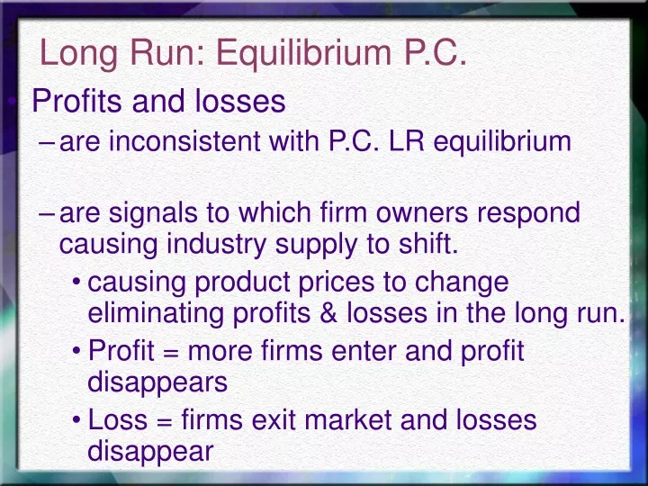
Long Run: Equilibrium P.C. Profits and losses are inconsistent with P.C. LR equilibrium are signals to which firm owners respond causing industry supply to shift. causing product prices to change eliminating profits & losses in the long run. Profit = more firms enter and profit disappears

E N D
Long Run: Equilibrium P.C. • Profits and losses • are inconsistent with P.C. LR equilibrium • are signals to which firm owners respond causing industry supply to shift. • causing product prices to change eliminating profits & losses in the long run. • Profit = more firms enter and profit disappears • Loss = firms exit market and losses disappear
Long Run Adjustment • 1.) Exit and Entry • stops when firms are making 0 economic profit. • 2.) Change Size of Plant • stops when firms have the plant that coincides with the min. LRATC and firms are making 0 economic profit
Long Run Adjustment S MC ATC d = MR P1 Price ($) Price ($) D q1 Q1 Quantity of Sweaters (firm) Quantity of Sweaters (industry) Entry & Exit Initial Market Condition Break-even P=Min.ATC
Long Run Adjustment S MC ATC d2 P2 Price ($) Higher price creates economic profit D2 D1 q1 q2 Q2 Quantity of Sweaters (industry) Entry and Exit Increased cold weather increases demand for sweaters d1 Price ($) P1 Q1 Q1 Quantity of Sweaters (firm)
Long Run Adjustment S1 MC S2 ATC d1 Price ($) Price ($) D2 D1 q1 Quantity of Sweaters (firm) Quantity of Sweaters (industry) Entry and Exit Economic profit attracts new firms. Price falls to break-even point. P1 Break-even P=Min.ATC Q1 Q1 Ease of Entry important for Long Run Adjustment
Long Run Supply S1 S2 Price ($) D2 D1 Quantity of Sweaters (industry) Constant Cost Industry Demand shifts, offering profit to current firms. LRS More firms enter, shifting supply yet not increasing input costs. P1 Long run supply is horizontal. Q1 Q1 Additional firms do not increase costs.
Long Run Supply S1 S2 Price ($) D2 D1 Quantity of Sweaters (industry) Increasing Cost Industry Demand shifts, offering profit to current firms. LRS More firms enter, shifting supply yet increasing input costs P1 Long run supply is upward sloping Q1 Q1 Additional firms increase costs.
Long Run Supply S1 S2 Price ($) D2 D1 Quantity of Sweaters (industry) Increasing Cost Industry Demand shifts, offering profit to current firms. More firms enter, shifting supply yet decreasing input costs P1 LRS Long run supply is downward sloping Q1 Q1 Additional firms decrease costs.
Technological Change: Process of Adjustment • The first firms to adopt new technology will make a profit, other firms will eventually exit or switch • Composition of industry is varied consisting of new and old tech firms • Technological change brings temporary gains to producers • Lower prices and better products resulting from technological advance bring permanent gains to consumers
Long Run Adjustment LRAC MC1 SRAC1 MR1 m Long-run competitive equilibrium Change Plant Size(Firm-wide) Changing plant size will Result in changed MC and Therefore SRAC curves 40 Short-run profit maximizing point MC0 SRAC0 Price (dollars per sweater) 25 MR0 20 14 6 8 Quantity (sweaters per day)
MC LAC SAC E Price per Unit d = MR = P = MC=SRATC =LRATC Qe Quantity per Time Period Long-Run: Competitive Equilibrium • P (= MR) = MC : SR equilibrium • MC = SRATC : no incentive for firms to enter or leave • Min LRATC : minimum per unit costs achieved so plant size is optimal In the Long Run: P=MC=minATC
Long Run: Summary • Competition and the Desire for Profit • The forces that provide for both productive and allocative efficiency in PC markets in the long run • P = MC = min ATC (P.C. Long Run Equil.) • Indicates both productive and allocative efficiency. Micro Efficiency and the Long Run
Productive Efficiency • Requires that each good in the optimal product mix be produced in the least costly way. • 1.) Productive Efficiency - occurs when • P = min ATC • firms produce at min ATC and receive a price =min ATC. Firms must use the best available, least-cost technology, or they will not survive.
Allocative Efficiency • Requires resources be allocated to firms so as to obtain the optimal mix of products • 2.)Allocative Efficiency - occurs when • P = MC • resources are used to produce the total output whose composition best fits consumer preferences, the optimal product mix.
Allocative Efficiency:P=MC Recall: Price of X • society’s measure of the relative worth of that product at the margin. • measures the extra benefit or value society gets from additional units of X (MSB – Marginal Social Benefit) Marginal Cost of X • society’s measure of the value of the other goods that the resources used in the production of an extra unit of X could otherwise have produced. • measures the sacrifice or opportunity cost to society of using resources to produce additional X(MSC – Marginal Social Cost)
Allocative Efficiency • When P = MC \MSB = MSC • each good is produced to the point at which • society’s value of the last unit = society’s value of the alternative goods sacrificed by its production.
Consumer + Producer Surplus is Maximized Consumer Surplus Allocative Efficiency, MSC=MCB Producer Surplus Efficiency of the Equilibrium Quantity MC, MB $ MSC B0 P* C0 MSB Quantity Q0 Q*
Allocative Efficiency • When P = MC \MSB = MSC • each good is produced to the point at which • society’s value of the last unit = society’s value of the alternative goods sacrificed by its production. • economic well being is maximized; that is, consumer surplus + producer surplus, is maximized
Summary: Perfect Competition &The Invisible Hand • Consumers and producers pursue their own self-interest and interact in markets. • Market transactions generate an efficient—highest valued—use of resources.
Usefulness of the Perfectly Competitive Model • It reduces the complexity of reality into manageable size • It highlights the idea of an efficient allocation & use of resources • It shows the role of prices, profits and competition in the market system
Usefulness of the Perfectly Competitive Model • Serves as a yardstick against which real-world market structures, resource allocation, prices, profits, competition and firm behaviour can be compared. • Acts as a guide to public policy and corrective action.
Failure of Perfect Competition • Inefficient resource allocation can lead to MARKET FAILURE (ie: externalities and public goods) • PC firm are too small to engage in extensive R&D, slowing technological growth (ie: Microsoft wouldn’t be making so many advances if it where in a PC market)
Monopoly a single seller of a product which has no close substitutes. Market power is the ability to influence the market price by influencing the total quantity offered for sale.
Characteristics of Monopoly 1. Single seller • firm & industry are the same 2. Unique product 3. Barriers to entry 4. Good will advertising 5. Price maker/searcher
Why do monopolies arise? • Barrier to Entry: something that prevents new firms from entering and competing • Key resources owned by a single firm. • Government grants exclusive right (eg. patent) to produce product . • Economies of Scale - Natural Monopoly: single firm can supply a product to an entire market at a lower per unit cost than could 2 or more firms. - Using economies of scale to predate and maintain monopoly power is illegal in Canada
Natural Monopoly 2 firms can supply 4 million kWh at 10 cents/kWh 4 firms can supply 4 million kWh at 15 cents/kWh • There are economies of scale over the relevant range of output. 1 firm can supply 4 million kWh at 5 cents/kWh 15 10 Price (cents per kilowatt-hour) 5 ATC Demand cuts LAC to the left of the min. LAC D 0 1 2 3 4 Quantity (millions of kilowatt-hours)
Pricing & Output Decision: Monopolist • Monopolists have the ability to influence the output price by choosing the output level. • The firm’s demand curve is the market demand curve. • A monopolist’s MR is always less than price (except for the first unit)
Marginal Revenue: Always Less Than Price P = $8 TR = $24 Area B (-) Demand curve = AR curve 8 7 P = $7 TR = $28 Loss = -$3 D Area A (+) Gain = $7 3 4 To sell 3 units, each unit sold for $8 To sell 4 units, each unit sold for $7 Lose $1/unit on 3 units or -$3 Gain $7 on the 4th unit or +$7 Net Gain (MR) = $4 (TR/ TO) Price of Electricity Quantity of Electricity per Time Period
Demand & Marginal Revenue To increase quantity sold the monopolist lowers selling price lowering price to sell an additional unit also lowers price on the previous units - which previously would have sold for more. D=AR MR Marginal revenue lies below D/AR for the monopolist P2 Price, and Marginal Revenue per Unit P1 P3 Q1 Q2 Q3 Quantity per Time Period
Monopoly: Profit Max. Decision Ed’s Costs of Showing Movie $ C Film rental 1800 Auditorium O Auditorium rental 250 holds 700 S Operator 50 people T Ticket takers 100 S TOTAL $2200
10 9 8 7 6 $ Per Ticket 5 4 3 2 1 0 100 700 200 300 400 500 600 800 900 1000 Tickets Per Week Ed’s Profit Maximizing Decision Costs Film Rental $1800 Auditorium 250 Operator 50 Ticket Takers 100 Total $2200 Demand (AR) What will Ed charge for admission to maximize profits?
Profit Maximizing Rule • PRODUCE ALL THOSE UNITS FOR WHICH MR MC. • All costs are sunk/fixed: • TC = $2200 • MC = $0 TC=$2200 MC=0 Look at demand for revenue information P Q TR MR Profit $ $ $ $ 7 300 2100 TR/ TOTR-TC 6 400 2400 3.00 200 5 500 2500 1.00 300 4 600 2400 -1.00 200 3 700 2100 -100
10 9 8 7 6 $ Per Ticket 5 4 3 2 1 0 100 700 200 300 400 500 600 800 900 1000 Tickets Per Week The Profit Maximizing Decision Profit Maximization MR MC MC = 0 MR = 0 Q* = 500 P* = $5.00 Demand (AR) MR TR $2500 TC $2200 Profit $300
Change Cost Conditions • Now suppose the distributor of the films changes the rental fee from a flat $1800 to $800 and $2.00 for every ticket sold. • TFC=$800 +$400 = $1200
Revenue InfoCost Info Demand FC = $1200 P,$’s Qn MR,$’s TC,$’s MC,$’s 7.00 300 1800 6.00 400 3.00 2000 2.00 5.00 500 1.00 2200 2.00 4.00 600 -1.00 2400 2.00
10 9 8 7 6 $ Per Ticket 5 Demand (AR) 4 MR 3 2 1 0 100 700 200 300 400 500 600 800 900 1000 Tickets Per Week The Profit Max Decision when MC = $2.00 Profit Maximization MR MC MC = 2 MR = 2 Q* = 400 P* = $6.00 Profit=$400 MC
Midterm #2 • 1 Hour in length • 50 questions multiple choice • Allocate 1 min. per question • Feel free to leave questions until end • Non-cumulative: Covers all TOPICS since first midterm