Download
1 / 16
180 likes | 372 Vues
Motion Planning Geometrical Formulation of the Piano Mover Problem. Configuration Space. Environment made of bodies: compact and connected domains of the Euclidean space . Body placement : translation-rotation composition Placement Space P. Obstacles : finite number of fixed bodies

E N D
Motion Planning Geometrical Formulation of the Piano Mover Problem
Configuration Space • Environment made of bodies: compact and connected domains of the Euclidean space • Body placement: translation-rotation composition • Placement Space P • Obstacles: finite number of fixed bodies • Subspace E of the Euclidean Space • Robot: (R,A) with R=(R1, R2, … Rm) and P m A • A: valid placements defined by holonomic links • Configuration: minimal parameterization of A • For c in CS, c(R) is the domain of the Euclidean space occupied by R at configuration c.
Configuration Space Topology • Topology on CS: induced by Hausdorff metric in Euclidean space • d(c,c’) = dHausdorff(c(R),c’(R)) • Path: continuous function from [0,1] to CS
Configuration • Admissible: c(R) int(E) = • Free: c(R) E = • Contact: c(R) int(E) = and c(R) E ≠ • Collision: c(R) int(E) ≠
Configuration • Admissible: c(R) int(E) = • Free: c(R) E = • Contact: c(R) int(E) = and c(R) E ≠ • Collision: c(R) int(E) ≠
Configuration • Admissible: c(R) int(E) = • Free: c(R) E = • Contact: c(R) int(E) = and c(R) E ≠ • Collision: c(R) int(E) ≠ Admissible Free Collision Contact
Configuration • int(Admissible) = Free • Admissible ≠ clos (int(Admissible) ) • Admissible ≠clos(Free) • Numerical algorithms work in Free Admissible Free Collision Contact
Path search • Any admissible motion for the 3D mechanical system appears a collision-free path for a point in the CSAdmissible • How to translate the continuous problem into a combinatorial one?
Cell Decomposition • Cell: domain of CSAdmissible • Cells C1 and C2are adjacent if: • clos (C1 ) C2 clos (C2 ) C1 ≠ • Connected components of topological space • = • Connected components of the cell graph
Cell Decomposition Ingredients • Cell decomposition algorithm • Algorithm to localize a point within a cell • Algorithm to move within a single cell • A path search algorithm within a graph • Examples: • Sweeping line algorithm to decompose polygonal environments into trapezoids • Cylindrical algebraic decomposition
Cell Decomposition • Sweeping line algorithm to decompose polygonal environments into trapezoids
Retraction • Almost everywhere continuous function from space S to sub-space retract (S) such that: • x and retract (x) belong to the same connected component of S • Each connected component of S contains exactly one connected component of retract (S) • Connected components of topological space • = • Connected components of the retracted space
Retraction • Apply retraction recursively to decrease the dimension of the topological space • Examples: • Voronoï diagrams • Visibility graphs • Retraction on the border of the obstacles (algebraic topology issues) • Probabilistic roadmaps
Retraction • Visibility Graph
Retraction • Voronoï Diagram