Download
1 / 13
130 likes | 143 Vues
Using the Calculator . 3.2 Residuals and the Least-Squares Regression Line. Using the Calculator – TI Series – p. 146. STAT Edit Enter data. x- variable in L1 y -variable in L2. Using the Calculator – TI Series – p. 146. L1: 2 nd , press 1 L2: 2 nd , press 2

E N D
Using the Calculator 3.2 Residuals and the Least-Squares Regression Line
Using the Calculator – TI Series – p. 146 • STAT Edit • Enter data. • x-variable in L1 • y-variable in L2
Using the Calculator – TI Series – p. 146 • L1: 2nd , press 1 • L2: 2nd, press 2 • Y1: VARS Y-VARS ↓ • 1: Function, Select 1: Y1 • STAT PLOT CALC • ↓ 8: LinReg(a+bx) • Press Enter
Using the Calculator – TI Series – p. 146 So the LSRL is: • Press Y= • Make sure Plot 1 is On with L1 & L2 for the x- and y-list • Press Enter
Using the Calculator – TI Series – p. 146 • Press Trace. • Going ← and → will help you jump from point to point • Going ↑ and ↓ helps you jump from the points to the line • Zoom 9 to graph
Using the Calculator – TI Series – p. 146 *Note: You must have completed the previous steps for this to work. To get the residual plot: • Press 2nd List (STAT button) • Select 7:RESID • Go to STAT PLOT • Go to Ylist
Using the Calculator – TI Series – p. 146 To get the residual plot: • Zoom 9 to graph
Using the Calculator – HP Prime – p. 146 • Enter data • x-variable in C1 • y-variable in C2
Using the Calculator – HP Prime – p. 146 • Press Symb • First box is x-variable (C1), Second box is y-variable (C2) • Make sure it says linear • Fit 1 should have M*X+B • Press Plot • Press Menu, then Fit to get the line
Using the Calculator – HP Prime – p. 146 ***NOTE: We would switch the equation around to be a + bx. So the LSRL is: • Go back go SYMB • Check out the equation
Using the Calculator – HP Prime – p. 146 To get residual plot: • Go to the Home Screen • Press the toolbox • Select App on the screen, go ↑ to Statistics 2Var → to 3 Resid • Press Enter • Type S1 (for Scatterplot 1), Sto► (bottom right corner of screen), then C3 • Press Enter
Using the Calculator – HP Prime – p. 146 To get residual plot: • Go to Numerical View • Residuals are listed in C3 • Go to Symbolic View • Uncheck S1 • Use S2 with C1 as the x and C3 as the y
Using the Calculator – HP Prime – p. 146 To get residual plot: • Press Plot • Press Menu (soft key on screen) and scroll to autoscale for better view