9. Model Atmospheres

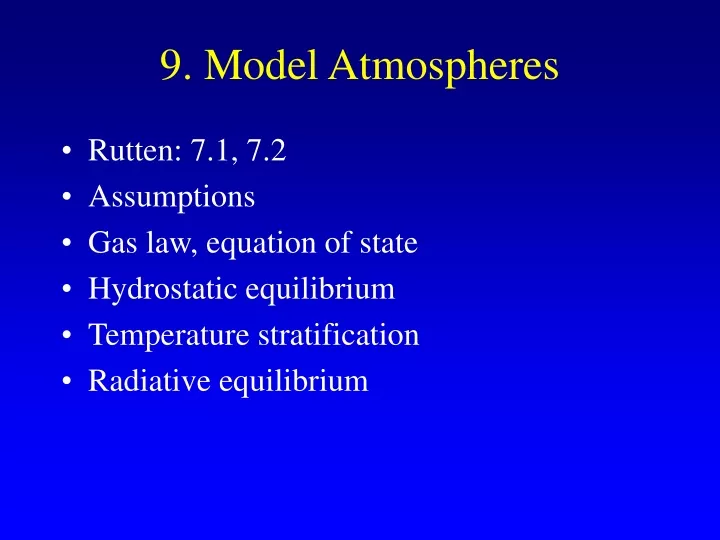
1. 9. Model Atmospheres • Rutten: 7.1, 7.2 • Assumptions • Gas law, equation of state • Hydrostatic equilibrium • Temperature stratification • Radiative equilibrium

2. Model Atmospheres Problem: Construct a numerical model of the atmosphere to estimate (a) Variation of physical variables (T, P) with depth (b) Emergent spectrum in continuum and lines Compare calculated spectrum with the real star and revise model until agreement is satisfactory. Calibrations: A grid of models varying Teff, g, and chemical composition can predict classification parameters such as colour indices and metal abundance indicators, and a main sequence of g vs Teff to compare with interior models.

3. Model Atmosphere Assumptions • Homogeneous plane parallel layers • Hydrostatic equilibrium • Time independent • Radiative Equilibrium • Local Thermodynamic Equilibrium

4. Plane Parallel: “Thickness” of photosphere << R* g constant throughout photosphere Adequate for main sequence stars, not for extended envelopes, e.g., supergiants Homogeneous: Physical quantities vary with depth only Reduces problem to one dimension Ignores sunspots, starspots, granulation,… Hydrostatic Equilibrium: Assume pressure stratification is such that balances g Ignores all movement of matter

5. Steady State: Properties do not change with time ERT assumed independent of time Energy level populations constant: detailed balance or statistical equilibrium Neglects: rotation, pulsation, expanding envelopes, winds, shocks, variable magnetic fields, etc Radiative Equilibrium: All energy transport by radiative processes Neglects transport by convection Neglects hydrodynamic effects There is much evidence for the existence of velocity fields in the solar atmosphere and mass motions, including convection, are significant in stellar atmospheres, particularly supergiants. A complete theory must include hydrodynamical effects and show how energy is exchanged between radiative/non-radiative modes of energy transport

6. Local Thermodynamic Equilibrium (LTE): All properties of a small volume of material gas are the same as their thermodynamic equilibrium values at the local values of T and P. A reasonably good approximation for photospheres of stars that are not too hot, or too large, as most of the spectrum is formed at depths where LTE holds.

7. Gas Law, Equation of State The ideal gas law generally holds in stellar photospheres. The classical version is: With nmole the number of moles, the gas constant R = kNA = k/mH. Other versions use total number density Ng = nmoleNA / V, mean “molecular” weight m = m/mH, density r = NgmmH: Total pressure is sum over all partial pressures Pg = S NikT. Partial electron pressure:

8. P(r + dr) dA r + dr Dm P P r P(r) GMDm / r2 Hydrostatic Equilibrium Hydrostatic equilibrium: acceleration negligible: Plane parallel: Optical depth dt0 = -k0rdz:

9. Simplest case of isothermal atmosphere with constant m and only gas pressure gives: Where the pressure scaleheight is HP = RT/mg. The solution is the standard barometric exponential decay law: Scaleheight indicates extent of atmosphere: spectra come from layers Spanning a few HP. For sun HP ~ 150 km, all photosphere ~ 500 km. Plane-parallel holds if HP / R* << 1. Holds for all except largest supergiants. Note this test does not say anything about horizontal inhomogeneities, and other effects that can mess up plane-parallel approximation.

10. Radiative Equilibrium From the Gray Atmosphere, the radiative equilibrium condition was that the flux was constant throughout the atmosphere: dF / dt = 0. Including frequency dependence we get a more rigorous condition: This says that all emitted energy must equal all extincted energy. It can also be written: In LTE, Sn = Bn(T[r]), so the above is solved to determine the temperature structure of an atmosphere.